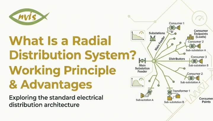
What Is a Radial Distribution System? Working Principle & Advantages

Posted on 27-07-2026 by Tushar Saluja

TL;DR

This blog is for engineering students, freshers, and anyone new to power systems who wants to understand how electricity actually travels from a substation to their home, explained in plain English before technical terms show up.
A radial distribution system sends power in one direction only, like a tree with a single trunk and branches, which makes it simple and cheap but leaves everyone downstream vulnerable if something breaks upstream.
You will learn exactly how a radial system is built, why it still powers most of rural and small town India despite being over a century old as a design, and where it genuinely struggles.
We will also break down the ring main system, which fixes the radial system’s biggest weakness by giving power a second path to travel, and compare both side by side.
By the end, you will understand not just definitions but actual engineering logic behind why utilities choose one system over another, plus where 2026’s smart grid technology is changing that choice.

A single garden hose connected to one tap illustrates the basic idea well. Water flows from tap, through hose, and outward to wherever it is directed. If that hose has smaller hoses branching off it, each watering a different flower bed, stepping on the main hose near the tap stops every branch downstream from receiving water immediately. Nothing resumes until that one blockage is cleared.

A radial distribution system works on essentially the same principle, except substance moving through the network is electricity, and the area being served is an entire town, industrial zone, or residential colony rather than a garden.

This design is one of oldest and most widely used methods of delivering electricity from a substation to homes and businesses. It is neither the most sophisticated nor most reliable system available, yet it has remained in use for over a century because it solves a specific practical problem effectively: distributing power to a large number of consumers at low cost and with minimal complexity.

This guide covers what a radial distribution system is, how it functions step by step, why it continues to be widely adopted, where its limitations lie, and how the ring main system was developed to address its central weakness. It also examines how rooftop solar adoption and smart grid automation are reshaping distribution design in 2026.

Understanding Power Distribution Before We Get Into Radial Systems

Before we zoom into the radial system specifically, it helps to understand the bigger picture it fits into.

Electricity does not travel directly from a power plant to your ceiling fan. It goes through a long relay race. Power plants generate electricity at very high voltages because that is the most efficient way to push electricity across long distances with minimal loss. This high voltage electricity travels through transmission lines, massive steel towers you see crossing highways and open fields, until it reaches a substation closer to where people actually live.

At substation, transformers step that voltage down to a level that is safer and more usable. From here, jobs shift to the distribution system, network of wires, poles, and transformers that carries electricity to homes, shops, and factories.

There are a few different ways engineers design this final stretch, and the layout they choose is called distribution topology. A radial system is one option. The ring main system is another. There is also an interconnected system, which is essentially a ring main powered by more than one substation. Each has its own tradeoffs around cost, reliability, and complexity, and understanding radial systems is really the foundation for understanding all of them.

What Is a Radial Distribution System

Now let us get specific. A radial distribution system is a layout where power flows from a single substation, out through feeder lines, and finally to individual consumers, with electricity moving in only one direction the entire time. There is no loop, no alternate path, and no second route for power to take if the main one gets blocked.

Go back to that garden hose picture. tap is your substation. The main hose is your primary feeder, thick cable that carries the bulk of electrical load. smaller branching hoses are lateral, secondary lines that peel off main feeder to serve specific streets, buildings, or neighborhoods. Water, or in this case current, only moves outward from the tap. It never flows back or sideways to find another route.

This is why the system is called “radial.” Think of a bicycle wheel. spokes radiate outward from the center hub in straight lines, each one independent of others. A radial distribution system radiates out from its substation in exactly the same way, with each feeder acting like its own spoke, unconnected to others.

How a Radial Distribution System Actually Works

Here is where pieces come together. A radial distribution system is built from four main components, and each one plays a distinct role in getting power from substation to your switchboard.

substation is the starting point. This is where high voltage electricity coming in from the transmission network gets stepped down to distribution level voltage by transformers. Think of this as a pressure regulator on our garden hose, it takes something too powerful to use directly and brings it down to a manageable level.

From substation, primary feeders carry this power outward. These are thick, high capacity lines designed to handle a large chunk of total electrical load, similar to that main garden hose carrying bulk of water flow.

Laterals branch off primary feeders to serve smaller, localized areas, a specific street, a housing block, or a single large building. This is where branching hoses come in, each one dedicated to a smaller piece of overall coverage area.

Finally, distribution transformers step voltage down one more time, from feeder level voltage to actual usable voltage that reaches your home’s wiring, typically 230V single phase or 415V three phase supply used across most of India.

Now here is the part that really defines a radial system: what happens when something goes wrong. Since power only flows in one direction, a fault, say a fallen tree branch snapping a line, anywhere along a feeder cuts off electricity to every single consumer downstream of that point. There is no rerouting, no backup path, no way for power to reach those consumers through a different route. Everyone past fault simply loses supply until repair crews physically fix the break.

This single direction, no backup design is both the radial system’s greatest strength and its biggest limitation, and understanding why requires looking at both sides.

Why Radial Distribution Systems Are Still So Widely Used

If losing power to an entire neighborhood because of one broken line sounds like a serious drawback, you might wonder why anyone still builds systems this way. The answer comes down to one word: economics.

A radial system is, hands down, the cheapest and simplest distribution layout to design, build, and maintain. It needs fewer cables, fewer switches, and far less protective equipment compared to more complex layouts. There is no loop to close, no need for sophisticated switching logic to figure out which direction power should flow. Engineers can plan and lay out a radial network relatively quickly, which matters enormously when you are trying to electrify a large rural area or a rapidly growing township without unlimited budget.

This is exactly why radial systems dominate in a few specific situations. Rural electrification is a classic case. In villages and small towns with lower population density and spread out homes, spending extra money on backup pathways rarely makes financial sense when an alternative, a simple radial line, gets the job done at a fraction of cost.

You will also find radial systems in peripheral urban and suburban feeders, edges of cities where load is scattered and reliability requirements are lower than in a dense city center. Individual industrial plants often use radial layouts internally for specific process areas or lighting circuits, where a brief outage is inconvenient but not catastrophic. And for temporary power supplies, like construction sites or mining operations, radial systems are almost always the default choice because mobility and speed of setup matter more than long term reliability.

Put simply, radial layouts still dominate distribution at voltages below 33kV, particularly for medium density residential areas, small commercial zones, and process load centers, because simplicity to cost ratio is hard to beat when uninterrupted supply is not top priority.

Real Limitations of a Radial Distribution System

Simplicity always comes with tradeoffs, and it is worth being honest about what those are before deciding whether a radial system fits your situation.

The most obvious weakness is low reliability. Because there is no alternative feeder or backup path, any fault anywhere along the line results in a complete supply failure for every consumer positioned after that fault point. If you live at the far end of a radial feeder and someone else’s transformer trips near the substation, your lights go out too, even though the problem has nothing to do with your part of the network.

There is also a voltage drop problem built into the physics of the system. As electricity travels further from substation, some voltage is inevitably lost along the way due to resistance in wires. This means consumers closer to the substation get a healthy, stable voltage, while those at the far end of a long feeder often experience noticeably lower voltage, especially during peak demand hours. Utility engineers have to size conductors carefully and place transformers strategically just to keep this voltage drop within acceptable limits.

Uneven loading is another consequence of layout. The section of distributor closest to the substation ends up carrying the heaviest current load, since it has to support everything downstream of it. This uneven distribution of electrical stress across networks is simply built into how radial systems are structured.

Finally, fault location can be genuinely difficult to pinpoint. When something goes wrong deep inside a sprawling radial network, technicians often have to physically trace line section by section to find exact break, which can mean longer outage times compared to systems with built in monitoring and isolation features.

None of these limitations make radial systems a bad choice. They simply define where the system makes sense and where it does not. And that brings us to a design that was created specifically to solve reliability problems.

Radial System vs Ring Main System: What Changes

If you take everything we just covered about radial systems and ask, “what if we gave power a second way to reach the same point,” you arrive at the ring main system.

A ring main distribution system is a closed loop configuration where the feeder starts at a substation, loops through the entire service area, and comes back to the same substation, forming a complete circle rather than a straight line with branches. Every distribution transformer along this loop is connected to two feeder paths instead of one.

Think back to our garden hose analogy, but now imagine the hose is a full circle instead of a single line with branches. Water can reach any point on that loop from two different directions. If you pinch the hose at one spot, water simply reroutes and flows to that same spot from another direction. Nothing downstream loses supply.

This is precisely what the ring main system achieves electrically. If a fault occurs anywhere along the ring, switchgear isolates just that faulty section, and every other consumer on loop continues receiving power from the opposite direction. This single design change fundamentally transforms the reliability equation.

How Ring Main System Works

mechanics of a ring main system are not dramatically different from a radial one at component level, transformers, feeders, and distribution equipment are all still present. What changes is topology, the way these components are connected together.

loop begins and ends at the same substation bus bar. Distribution transformers are tapped at various points around this loop rather than sitting at the end of a dead end branch. Ring Main Units (RMUs) are compact switchgear installed at tap-off points. Working together with protective relays and circuit breakers, they isolate faulty sections while keeping the remaining network energized.

When a fault occurs somewhere on a ring, protective devices like circuit breakers and relays detect exactly where the problem is and isolate only that specific segment. Power continues flowing to every other consumer through the opposite side of the loop. Once repair crews fix faulty sections, it gets reconnected, and the ring returns to its normal closed loop state.

This closed loop structure also solves voltage drop and uneven loading problems that plague radial systems. Since every point on the ring can potentially receive power from two directions, electrical loading can be shared between two supply paths, depending on the network configuration and operating conditions. Voltage fluctuations at any given consumer’s terminal are also significantly reduced, because power is essentially arriving from both sides rather than weakening steadily along one long single direction line.

Radial vs Ring Main: A Direct Comparison

Factor	Radial Distribution System	Ring Main Distribution System
Power flow direction	Single direction only	Can flow from either direction
Initial cost	Low	Higher, due to extra cable and switchgear
Reliability	Low, one fault cuts supply to everyone downstream	High, faults are isolated without a full outage
Voltage drop	Significant at far end of long feeders	Minimal, load is balanced across loop
Maintenance	Requires full shutdown of affected section	Sections can be isolated while rest stays powered
Fault location	Harder to trace, longer repair time	Easier to isolate using RMUs and protective relays
Best suited for	Rural areas, small towns, temporary supply, low density zones	Cities, hospitals, industrial parks, data centers, anywhere continuous power matters

Neither system is universally “better.” The right choice depends entirely on what specific area needs. A rural stretch with scattered homes rarely justifies extra cost of a ring main. A hospital or a data center, on other hand, cannot afford the kind of prolonged outage a radial fault would cause, making ring main’s higher upfront cost an easy trade to accept.

Radial Distribution Systems in Age of Smart Grids

Here is something worth understanding as you head into 2026 and beyond: the way engineers think about radial systems is shifting, even if underlying wiring often stays the same.

Two big forces are reshaping distribution design right now. First is distributed generation, a term that basically means power sources that are not traditional centralized power plants. Rooftop solar panels, small battery storage systems, and even electric vehicles feeding power back into the grid are becoming common, especially as adoption accelerates across Indian households and businesses. A traditional radial system was designed around the assumption that power flows in exactly one direction, from substation to consumer. When a home with rooftop solar starts pushing power back into the grid during sunny hours, that one directional assumption starts to break down, and utilities have to rethink how their radial feeders handle this reverse flow.

The second force is grid automation, and this one is a genuinely exciting shift. Distribution networks in 2026 are increasingly using sensors, real-time monitoring, and automated switching to detect faults, isolate the affected section, and restore supply to healthy sections within seconds where feeder automation is available, often before a technician is even dispatched. This is sometimes called a self-healing grid. Even within a fundamentally radial layout, adding automated sectionalizing switches, tie switches, and remote monitoring can dramatically cut outage times, closing some of the reliability gap that traditionally only a ring main system could offer.

None of this means radial systems are disappearing. For low density rural areas and temporary installations, core economics still favor a simple radial layout. What is changing is the layer of intelligence sitting on top of that layout, using data and automation to make even a basic radial network respond faster and smarter when something goes wrong.

Conclusion

A radial distribution system is, at its core, a straightforward idea: send power outward from a single source, branch by branch, in one direction. That simplicity is exactly why it has powered rural electrification, small towns, and temporary installations for over a century, and why it remains practical, budget friendly choice wherever high reliability is not top priority.

But that same simplicity is also its biggest weakness. A single fault anywhere along a line can cut power to everyone downstream, voltage naturally drops the further you travel from substation, and locating faults can take time. The ring main system exists precisely to solve this problem, giving power a second path so that a fault in one section does not mean an outage for everyone else on the network.

As you continue exploring electrical engineering, whether for coursework, competitive exams like GATE or SSC JE, or genuine curiosity about how grid around you actually works, understanding radial and ring main systems gives you a solid foundation for grasping more advanced topics like interconnected systems, smart grid automation, and growing role of distributed generation in reshaping how power reaches our homes.

FAQs

What is the main difference between a radial and a ring main distribution system?

A radial distribution system sends power in a single direction from substation to consumers with no backup path, while a ring main distribution system forms a closed loop, allowing power to reach any point from two directions and continue supplying consumers even if one section develops a fault.

Why is the radial distribution system still used if it is less reliable?

It remains widely used because it is significantly cheaper to install and simpler to maintain than alternatives like ring main systems, making it a practical choice for rural areas, small towns, and temporary power supplies where high reliability is not the primary concern.

What happens when a fault occurs in a radial distribution system?

Since power flows in only one direction with no alternate route, a fault anywhere along the feeder cuts off supply to every consumer positioned downstream of that fault point until repair crews physically locate and fix the break.

Is the ring main system always better than the radial system?

Not necessarily. A ring main system offers much higher reliability and better voltage stability, but it also costs significantly more to install due to extra cabling and switchgear required, so radial systems are still a more economical choice for low density or budget constrained areas.

What is a Ring Main Unit and how does it relate to the ring main system?

A Ring Main Unit (RMU) is a compact switchgear unit used in ring main distribution systems. It works with protective devices to isolate faulty sections while allowing the rest of the loop to remain energized, minimizing power interruptions to unaffected consumers.

How is smart grid technology changing radial distribution systems?

Modern grid automation is adding sensors and automated switching to radial networks, allowing faults to be detected and isolated within seconds rather than requiring a technician to manually trace lines, which is narrowing the reliability gap between radial and ring main systems even without a full topology change.

Tags: Radial Distribution System

Ring Main Distribution System: Working Principle, Advantages, and Why It Powers Modern Cities

Posted on 25-07-202625-07-2026 by Tushar Saluja

TL;DR

This blog is for engineering students, freshers, and anyone curious about how electricity reaches homes and factories without cutting off during repairs. It explains ring main distribution systems in plain language, starting from basics.
A ring main system connects distribution points in a closed loop instead of a single dead end line, so power can reach every point from two directions.
If one section of the loop develops a fault, engineers isolate just that section while the rest of the loop keeps running normally.
India’s DISCOMs are actively modernizing distribution networks under the RDSS scheme, with SCADA monitoring, digital substations, and, where applicable, smart Ring Main Units and SF6-free switchgear being deployed as part of network upgrades.
Understanding ring main systems opens doors to real careers in power distribution, smart grid technology, and utility engineering, with fresher salaries typically starting between 3.5 LPA and 7 LPA in India.

Also read,

Picture a city with only one road leading into it. If that road gets blocked for repairs, nobody gets in or out until it reopens. Now picture the same city with a ring road circling it, connected at multiple points. Block one section, and traffic simply flows around it through the other side. Nobody is stuck.

That is essentially the idea behind a ring main distribution system, just applied to electricity instead of traffic. It is one of the most important concepts in power systems engineering, and if you are studying electrical engineering or just curious about how lights in your hostel room stay on even when a utility crew is working nearby, this is a topic to understand.

In this guide, we will build up concepts from scratch. No assumed knowledge, no jargon dropped without explanation. By the end, you will understand what a ring main distribution system is, how it actually works, why it matters more in 2026 than ever before, and what career paths open up if this field interests you.

What Is Electricity Distribution, and Why Does It Need a “System” at All?

Before getting into ring main systems specifically, let’s zoom out for a second.

Power plants generate electricity far away from where most of us live. That electricity travels through high voltage transmission lines over long distances, and then gets stepped down through substations before it finally reaches your street, your building, and your switchboard. This last stretch, from substation to your actual plug point, is called a distribution system.

Now here’s a question every distribution engineer has to answer: how do you lay out wires connecting substations to hundreds or thousands of consumers, in a way that is reliable, cost effective, and doesn’t leave everyone in the dark every time something goes wrong?

There are a few ways to design this layout. Two most common ones you’ll encounter as a student are the radial system and the ring main system. Understanding the radial system first actually makes the ring main system click much faster, so let’s start there.

Radial System: Simple, but Fragile

Think of a radial distribution system like a tree. There’s one trunk (substation), and branches spread out from it to reach different areas. Power flows in a single direction, from source outward, with no loops or alternate paths.

This design is genuinely appealing on paper. It’s simple to plan, cheap to build, and easy to understand. For a small town or a rural area with modest power needs, a radial layout does the job well enough.

But here’s the catch. Because there’s only one path from source to any given consumer, a fault anywhere along that path cuts off everyone downstream from it. If a cable snaps two kilometers from the substation, every consumer beyond that point loses power immediately, and stays without power until the fault is physically located and repaired.

This is exactly the “one road into the city” problem we talked about earlier. It works fine until something breaks, and then it breaks badly.

Ring Main Distribution System: What It Actually Is

A ring main distribution system solves the radial system’s biggest weakness by doing something clever: instead of ending the distribution line at the last consumer, it loops it back to the starting point (or connects it to another substation), forming a closed ring.

In more technical terms, a ring main distribution system is a distribution network where a feeder starts from a substation, passes through various load points or distribution transformers, and returns to the same substation bus (or an adjacent one), forming a continuous loop with no dead end.

Every distribution transformer or tap off point along this ring is now connected to two sides of the loop, not just one. This means each point can receive power from either direction. If a fault occurs anywhere in the ring, engineers can isolate that specific faulty section using switches and circuit breakers, and the rest of the ring keeps supplying power normally, just from the opposite direction.

This single design choice, the closing loop, is what makes the ring main system so much more reliable than the radial system, and it’s the reason many urban and industrial distribution networks in India use some form of ring main configuration today.

How a Ring Main System Actually Works: Step by Step

Let’s walk through the working principle slowly, because this is where most explanations either skip steps or drown you in terminology too early.

Step 1: Power leaves substation in a loop. Instead of one feeder cable running in a straight line, the feeder cable leaves the substation, travels through the service area, and comes back to the same substation (or connects to a neighboring one). This closed path is “ring.”

Step 2: Distribution points tap into the ring. At various points along this ring, distribution transformers are connected. These transformers step voltage down further so it’s usable for homes, shops, and smaller industrial loads. Each transformer is connected to the ring from both directions, allowing supply to be restored from the alternate side if one section is isolated.

Step 3: Switches and circuit breakers sit at key points. This is the part that makes fault isolation possible. Circuit breakers and switches (often bundled together in a compact unit called a Ring Main Unit, or RMU, which we’ll cover shortly) are installed at strategic points around the ring. These devices can open or close specific sections of the loop on command.

Step 4: A fault occurs somewhere in the ring. Let’s say a cable fault develops between two tap off points. Protection relays detect abnormal current flow almost instantly and trigger nearest circuit breakers to open, isolating just that faulty section.

Step 5: After the faulty section is isolated, supply to the healthy sections is restored either automatically through network automation systems or manually by utility operators, depending on the level of automation. Because every load point had two supply paths to begin with, the moment a faulty section is isolated, the unaffected part of the ring continues delivering power, just fed from the opposite direction. In modern automated systems, this rerouting happens within seconds. In older manual systems, a technician would locate faults and physically operate switches to restore supply to healthy sections.

Step 6: fault gets repaired, and ring is restored. Once a faulty cable section is fixed, isolated switches are closed again, and the ring returns to its normal closed loop operation.

That’s the entire working principle. No single point of failure can take down the whole network, because every load point was never dependent on just one path in the first place.

Ring Main Unit (RMU): Component That Makes It All Work

You’ll hear the term “Ring Main Unit” or RMU constantly once you start reading about ring main systems, so let’s clear this up properly.

An RMU is a compact, factory built, sealed switchgear unit that combines switches, circuit breakers, and protection devices needed at each tap off point on the ring, all inside a single enclosure. Instead of installing separate switches, breakers, and protection relays as individual pieces of equipment, utilities install one RMU that does all of it in a much smaller footprint.

In India, RMUs are typically used in the 11kV to 33kV range, which covers most secondary distribution networks in cities, industrial parks, and large residential complexes. A standard RMU usually has two ring feeder units, connecting to either side of the loop, and one transformer feeder unit that supplies local distribution transformers.

RMUs matter for a practical reason: they make ring main systems genuinely deployable in dense urban areas. Since RMUs are compact and can be installed both indoors and outdoors with minimal maintenance, they’ve become standard building blocks for ring networks in Indian cities where space is always at a premium.

Advantages of Ring Main Distribution System

Now that you understand how it works, advantages should already make intuitive sense. Let’s go through them properly, because these show up frequently in exams and interviews alike.

Higher reliability through redundancy. This is a headline advantage. Since every load point has two possible supply paths, a single fault doesn’t cause a widespread blackout. Only a specific faulty section gets isolated, and it can serve a very small area, sometimes just stretching between two RMUs.

Better voltage regulation. In a radial system, consumers far from substation often experience noticeable voltage drops, especially during peak load hours. In a ring system, because loads are fed from both directions, voltage stays more stable across the entire network. Ring main systems generally provide better voltage regulation than comparable radial systems because loads can be supplied from multiple directions, which is a meaningful improvement over comparable radial setups.

Reduced power losses. Ring main systems can reduce voltage drops and, in some network configurations, lower distribution losses through improved load sharing. However, the actual reduction depends on network design and operating conditions, which translates to better overall efficiency.

Easier maintenance without full shutdowns. Maintenance crews can isolate a specific section of the ring for planned work while the rest of the network stays live. This is enormously valuable for industries and facilities that cannot afford any downtime, like hospitals, data centers, pharmaceutical plants, and continuous manufacturing lines.

Scalable for future growth. As a city or industrial area expands, new distribution transformers and tap off points can be added to existing rings without redesigning the whole network. This modularity is a major reason ring systems are preferred for growing urban centers and industrial parks.

Disadvantages You Should Also Know

No system is perfect, and exam questions love asking about limitations just as much as advantages.

Higher initial cost. Building a closed loop requires more cable length, more switchgear, and more protective devices compared to a simple radial layout. redundancy that makes ring systems reliable also makes them more expensive to build.

More complex protection scheme. In a radial system, fault current only flows in one direction, so protection design is relatively straightforward. In a ring system, fault current can arrive from either side, which means protection relays need to be directional, and coordinating them correctly across the whole loop takes careful engineering.

More components mean more potential failure points. Ironically, while ring design reduces impact of any single fault, it introduces more equipment (breakers, RMUs, relays) that could individually fail. Good design and maintenance practices are essential to keep this from becoming a real problem.

Planning and design complexity. Laying out an efficient ring, especially one connecting multiple substations, takes more careful planning than a straightforward radial layout. This isn’t usually a dealbreaker, but it does mean more engineering hours upfront.

Ring Main vs Radial Distribution System: A Quick Comparison

Aspect	Radial System	Ring Main System
Supply path	Single path from source to load	Two paths available for every load point
Reliability	Low; one fault can black out everyone downstream	High; faulty section isolates without affecting rest
Voltage regulation	Poor at far ends of feeder	Better across entire loop
Initial cost	Lower	Higher, due to extra cabling and switchgear
Protection complexity	Simple, unidirectional	More complex, needs directional relays
Best suited for	Small towns, rural areas, low density loads	Cities, industrial parks, critical facilities

Ring Main Systems in India: 2026 Update

Here’s where things get genuinely current, and this is worth paying close attention to if you’re a student trying to understand where this field is heading.

India’s electricity distribution sector has been undergoing a massive modernization push under the Revamped Distribution Sector Scheme (RDSS), a Government of India initiative launched in 2021. Under the scheme, distribution infrastructure projects worth over ₹2.83 lakh crore have been sanctioned, including ₹1.53 lakh crore for loss reduction infrastructure and ₹1.31 lakh crore for smart metering. The loss reduction works include feeder segregation, substation augmentation, new substations, distribution transformer upgrades, and SCADA/DMS systems for real-time monitoring. These investments are modernizing distribution networks across the country, with technologies such as Ring Main Units (RMUs) being deployed where appropriate to improve reliability and operational efficiency.

The numbers here are worth sitting with for a moment. India’s Aggregate Technical and Commercial losses, a measure of how much power gets lost or unaccounted for in the distribution network, dropped significantly over recent years due to a combination of infrastructure upgrades, improved metering, network modernization, and operational reforms. That is a meaningful improvement, and ring main upgrades are one of several factors contributing to these improvements, alongside better metering, feeder segregation, and distribution automation.

On the technology side, RMUs themselves are evolving fast. Traditional RMUs used SF6 gas as an insulating medium, but SF6 has a very high global warming potential, and industry is actively shifting toward SF6 free alternatives using solid dielectric or vacuum based insulation. Schneider Electric has already run pilot projects using SF6 free “AirSeT” technology in Mumbai and Delhi, reporting significantly lower carbon footprints compared to traditional gas insulated units.

Smart RMUs are also becoming standard in new installations. These units go beyond basic switching by integrating remote monitoring, automated fault detection, and communication with SCADA and Distribution Management Systems. In practice, this means faults that once took a technician driving to a site and manually operating switches can now be detected and isolated remotely within seconds, dramatically cutting outage times.

For a student entering this field today, this matters because the main system you learn in your textbook is no longer purely mechanical and manual. The version being deployed on ground right now is increasingly digital, automated, and connected, and that shift is only accelerating.

Applications of Ring Main Distribution Systems

Ring main systems aren’t just a theoretical concept confined to textbooks. Here’s where you’ll actually encounter them in the real world.

Urban and city power distribution. Many urban areas in India use ring main networks, particularly in commercial districts, industrial areas, and high-reliability distribution zones, particularly in dense commercial and residential zones where reliability expectations are high.

Industrial parks and manufacturing facilities. Factories running continuous processes, especially in sectors like pharmaceuticals and food processing, depend on ring systems to avoid costly production stoppages from power interruptions.

Large commercial complexes. Office towers, shopping malls, and IT parks with multiple zones and varying load profiles benefit from load balancing and reliability that ring systems provide.

Critical infrastructure. Hospitals, data centers, and telecommunications facilities, where even brief outages can have serious consequences, are prime candidates for ring main deployment.

Renewable energy integration. As solar and wind installations become more common, RMUs are increasingly used to connect these distributed energy sources into the grid, since their switching flexibility helps manage variable power flows more effectively.

Career Opportunities: Why This Topic Matters for Your Future

If you’ve made it this far, you might be wondering how understanding ring main systems actually translates into a career. Here’s an honest picture.

Power distribution is a genuinely stable, in demand field within core electrical engineering, and it’s only growing as India continues its grid modernization push. Roles you could realistically target after graduation include Distribution Engineer, Substation Engineer, Protection and Control Engineer, and Grid Automation Engineer, working either directly with state DISCOMs (like UPPCL, MSEDCL, or BESCOM) or with equipment manufacturers and engineering firms such as Schneider Electric, Siemens, ABB, and various power system consultancies.

On the salary front, fresher roles in power distribution engineering in India typically start somewhere between 3.5 LPA and 7 LPA, depending on company, location, and whether the role is with a utility, an OEM, or an EPC contractor. With a few years of experience, distribution and power systems engineers commonly move into the 7 LPA to 12 LPA range, and specialized roles involving SCADA, protection coordination, or grid automation can push well beyond that.

skills that matter most here are a solid grasp of power system fundamentals (exactly what we’ve covered in this article), familiarity with design and simulation tools like AutoCAD and ETAP, and increasingly, comfort with SCADA and Distribution Management System platforms as the sector digitizes. If you’re preparing for competitive exams like GATE, SSC JE, or state AE/JE recruitment, ring main systems and their comparison with radial systems are recurring, high yield topics, so effort you put into understanding this concept deeply pays off twice: once for your exams, and once for your actual career.

Conclusion

The ring main distribution system exists because of one simple engineering insight: a network with only one path to every destination is fragile, and closing that path into a loop creates redundancy that pays for itself the moment something goes wrong. From that single idea flows everything else we’ve covered, better voltage regulation, easier maintenance, higher reliability, and a genuine ability to scale as cities and industries grow.

What makes this topic worth your time right now, in 2026, is that it isn’t a static, settled concept. India’s distribution sector is actively rebuilding itself around smarter, more automated versions of exactly this technology, backed by serious government investment and real infrastructure targets. Whether you’re studying this for an exam, a project, or because you’re seriously considering a career in power systems, understanding ring main systems properly gives you a foundation that connects directly to what’s happening in the Indian power sector today, not just what’s printed in a decade old textbook.

FAQs

What is the main difference between a ring main system and a radial system?

A radial system has a single path from substation to each consumer, so a fault anywhere along that path cuts off everyone downstream. A ring main distribution system loops the feeder back to the source, giving every load point two possible supply paths, which means a fault only affects a small isolated section instead of the whole network.

What is a Ring Main Unit (RMU) used for?

An RMU is a compact, sealed switchgear unit that combines switches, circuit breakers, and protection devices at each tap off point on a ring main system. It allows operators to isolate faulty sections of the ring, connect distribution transformers, and maintain supply through alternate paths, all from a single, space efficient enclosure.

Why is ring main distribution system considered more reliable than other systems?

Reliability comes from redundancy. Because every point on the ring can be fed from two directions, isolating a fault in one section doesn’t interrupt supply to the rest of the network. This is fundamentally different from a radial system, where any fault downstream of a break leaves every subsequent consumer without power until repairs are complete.

What voltage levels are typically used in ring main systems in India?

In India, ring main systems and their associated RMUs are most commonly used in the 11kV to 33kV range, which covers secondary distribution networks serving cities, industrial areas, and large residential or commercial complexes. This falls within India’s medium voltage classification under CEA regulations.

Is SF6 gas still used in Ring Main Units, or is that changing?

SF6 gas has traditionally been a standard insulating medium in RMUs due to its excellent insulating properties, but because it has a very high global warming potential, industry is actively moving toward SF6 free alternatives using solid dielectric or vacuum based insulation. Utilities and manufacturers, including pilot projects in Indian cities like Mumbai and Delhi, are already deploying these greener alternatives.

What career paths open up if I understand ring main distribution systems well?

A strong grasp of ring main systems is directly relevant to roles like Distribution Engineer, Substation Engineer, Protection and Control Engineer, and Grid Automation Engineer. These roles exist both within state DISCOMs and at private companies like Schneider Electric, Siemens, and ABB, with fresher salaries in India typically starting between 3.5 LPA and 7 LPA and growing steadily with experience and specialization.

Tags: ring main distribution system

Two Wattmeter Method of Three Phase Power Measurement: Complete Guide

Posted on 21-07-202622-07-2026 by Tushar Saluja

TL;DR

This guide is written for engineering students, freshers, and GATE, SSC JE, and RRB JE aspirants who need a clear, exam ready understanding of two wattmeter methods for measuring power in three phase circuits.
The two wattmeter method uses only two wattmeters, not three, to measure total power in a three phase system, regardless of whether load is balanced or unbalanced, star connected or delta connected.
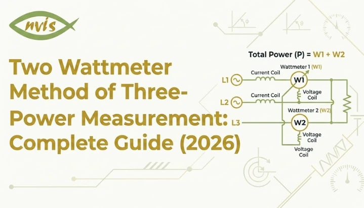
two core relationships are P = W1 + W2 for total power, andφ = tan⁻¹√3(W1−W2)/(W1+W2) for power factor angle in a balanced load.
Wattmeter readings change character with power factor: both readings are equal at unity pf, one wattmeter reads zero at 0.5 lagging pf, and one wattmeter reads negative below 0.5 pf.
This method remains a core skill for testing, commissioning, protection, and instrumentation engineers in India’s power sector in 2026, and it is distinct from consumer smart metering rollout under RDSS, which measures energy for billing rather than power for engineering analysis.

Also Read,

The two wattmeter method is a standard technique used in electrical engineering to measure total power in a three phase, three wire system using only two wattmeters instead of three. Also referred to as 2 wattmeter method in many textbooks and lab manuals, it works for both balanced and unbalanced loads, and for both star and delta connected systems, which is why it remains one of most widely used measurement techniques in power system testing, laboratory experiments, and competitive exam syllabi across India. This guide builds concepts from the ground up. It starts with what a wattmeter actually measures, moves into how two wattmeters are connected in a three phase circuit, derives two wattmeter method formula step by step, and works through a complete numerical example. It then covers how wattmeter readings behave at different power factors, where method is applied in real power systems, its practical limitations, and how this classical method connects to digital instrumentation and smart metering landscape shaping India’s power sector in 2026. A dedicated section also maps out career paths and salary expectations for engineering students who build expertise in this area.

What Is a Two Wattmeter Method?

A wattmeter is an instrument that measures real power, also called active power, in an electrical circuit. It does this by combining two measurements at once: the current flowing through the circuit and the voltage across it. Internally, a wattmeter has two coils. The current coil is connected in series with the circuit, so the same current that flows through the load also flows through this coil. The pressure coil, also called the voltage coil, is connected in parallel across the circuit to sense voltage. A wattmeter’s needle or digital display indicates the product of these two quantities, adjusted for the phase angle between them, to show the actual power being consumed. The two wattmeter method is a standard technique used to measure the total active power in a three-phase, three-wire system using only two wattmeters instead of three. It works for both balanced and unbalanced loads, as well as for both star (Y) and delta (Δ) connected systems, making it one of the most widely used methods for three-phase power measurement in laboratories and industrial power systems.

Why Three Phase Systems Need It?

In a single-phase circuit, one wattmeter is enough because there is only one phase to measure. A three-phase circuit is more complex because it has three separate phases, and in principle, each phase requires its own power measurement. In a three-phase, four-wire system with an accessible neutral conductor, three wattmeters connected between each phase and the neutral can directly measure the total power. Most industrial and power distribution systems, however, are three-phase, three-wire systems without an accessible neutral. In such systems, Blondel’s theorem states that the total power can be measured using one fewer wattmeter than the number of wires. Since a three-wire system has three conductors, only two wattmeters are required to measure the total active power accurately. This is the fundamental principle behind the two wattmeter method, allowing it to measure total power correctly for both balanced and unbalanced three-phase loads.

Two Wattmeter Method Circuit Connection

The physical connection of two wattmeters follows a consistent rule regardless of whether load is star connected or delta connected. Current coils of two wattmeters are connected in series with any two or three line conductors, commonly labelled R and Y, or A and B, depending on the naming convention used. No current coil is connected to the third line, commonly labelled B or C. Pressure coils of both wattmeters are then connected between the line carrying their respective current coil and the third, unmeasured line. In other words, one wattmeter’s pressure coil spans between line R and line B, while the other spans between line Y and line B. This means both pressure coils share a common connection point on the third line, even though no current coil is placed there.

Star (Y) Connected Load

In a star connected system, the load’s three phases meet at a common neutral point, but this neutral point is typically not accessible or not used in a three wire supply. Two wattmeters are connected exactly as described above, with their current coils in two of three lines and their pressure coils referenced to the third line. The absence of a neutral connection does not affect the accuracy of the method, since two wattmeter methods are designed specifically to work without one.

Delta (Δ) Connected Load

In a delta connected system, there is no neutral point at all, since each phase winding connects directly between two line conductors. The two wattmeter method applies here in exactly the same way as it does for a star connected load, because the method depends only on three line conductors, not on how the load’s internal windings are arranged. This is one of the practical advantages of the method: the same two wattmeter connection setup works whether the underlying load is star or delta connected, and the engineer performing the test does not need to know the internal configuration in advance.

Two Wattmeter Method Formula and Derivation

Two wattmeter method formulas can be derived by analyzing a balanced three phase star connected inductive load. Consider a balanced system where phase voltage magnitude is V, line current magnitude is I, and load has a lagging power factor angle of φ between each phase voltage and its corresponding phase current. Each wattmeter measures the product of a line current, a line voltage, and cosine of angle between them. Using standard phasor analysis, current in wattmeter W1 lags its reference line voltage by an angle of (30° minus φ), while current in wattmeter W2 lags its reference line voltage by an angle of (30° plus φ). Since both wattmeters are referenced to line voltages of equal magnitude VL and carry line currents of equal magnitude IL in a balanced system, their individual readings work out to: W1 = VL IL cos(30° φ) W2 = VL IL cos(30° + φ) Adding these two expressions and simplifying using standard trigonometric identities produces a clean result. angle terms combine in such a way that sum equals: W1 + W2 = √3 VL IL cos φ This expression is exactly standard formula for total power in a balanced three phase system, confirming that sum of two wattmeter readings gives correct total active power, written as: P = W1 + W2 The individual readings can also be used to extract power factor angle without needing to measure it separately. Subtracting two wattmeter expressions and dividing by their sum removes the VL IL term and leaves only trigonometric functions of φ. Working through this algebra gives power factor angle formula: φ = tan⁻¹ [√3 (W1 W2) / (W1 + W2)] Once φ is known, the power factor itself is simply cos φ. This derivation assumes a lagging power factor and a balanced load. For an unbalanced load, sum W1 + W2 still gives correct total power, but power factor angle formula above does not apply, since power factor is only a meaningful single value for a balanced three phase load.

Two Wattmeter Method Numerical Example

A numerical example makes measurement of three phase power by two wattmeter methods easier to apply in practice. Consider a balanced three phase load connected to a 400 V line to line supply, drawing a total power of 10 kW at a lagging power factor of 0.8. The first step is to find the power factor angle. Since power factor is 0.8, φ = cos⁻¹(0.8), which works out to approximately 36.87°. The next step uses the power factor angle formula in reverse. Rearranging φ = tan⁻¹[√3(W1 W2)/(W1 + W2)] gives: tan φ = √3 (W1 − W2) / (W1 + W2) Since W1 + W2 = P = 10 kW, and tan(36.87°) is approximately 0.75, substituting these values gives: 0.75 = √3 (W1 W2) / 10 Solving this equation gives the difference between the wattmeter readings: W1 − W2 ≈ 4.33 kW. With two equations now available, W1 + W2 = 10 kW and W1 − W2 = 4.33 kW, solving simultaneously gives W1 = 7.165 kW and W2 = 2.835 kW. These two values represent what an engineer would actually observe on two wattmeter displays during a real test on this load. Adding them back together confirms total power of 10 kW, and the difference between them reflects the load’s lagging power factor of 0.8. This same step by step approach applies to any balanced three phase power measurement problem, and it is the method most frequently tested in GATE Electrical Engineering and SSC JE Electrical numerical questions.

Wattmeter Readings at Different Power Factors

The relationship between two wattmeter readings and the load’s power factor is not linear, and it produces several distinct patterns that are important to recognize, both for practical testing and for exam preparation. The table below summarizes how readings behave across the power factor range for a balanced lagging load.

Power Factor	Angle φ	Wattmeter Behavior
Unity (1.0)	0°	Both wattmeters read exactly equal values; each shows half total power.
Above 0.5 lagging	0° to 60°	Both wattmeters read positive, but unequal, values; W1 reads higher than W2.
Exactly 0.5 lagging	60°	One wattmeter (W2) reads exactly zero; the other reads full total power.
Below 0.5 lagging	60° to 90°	lower reading wattmeter (W2) becomes negative; its terminals must be reversed to obtain a reading, and this value is then subtracted rather than added.
Zero (purely reactive)	90°	Both wattmeters read equal and opposite values, and sum correctly shows zero real power.

The case at 0.5 lagging power factor deserves particular attention, since it is one of most commonly tested scenarios. At this exact power factor, angle φ equals 60°, which makes angle term (30° minus φ) in wattmeter expression equal to negative 30°. Since cosine of negative 30° is a positive value, this wattmeter still reads a value, but companion expression works out so that one of two wattmeters reads exactly zero. This is not a fault or a wiring error; it is an expected mathematical outcome at that specific power factor. Below 0.5 lagging power factor, angle (30° plus φ) exceeds 90°, which makes its cosine negative. In practice, this means the pointer of an analog wattmeter would try to deflect backward, and standard procedure is to reverse connections of either current coil or pressure coil on that wattmeter to obtain a positive reading, then treat that reading as negative in calculation. Digital wattmeters typically display this as a negative value directly without requiring manual reversal. A separate limitation worth noting at this stage is that the two wattmeter method, by itself, cannot indicate whether the power factor is leading or lagging. The formula produces the same magnitude of φ for a leading load as it does for a lagging load with same wattmeter readings, since mathematics only reveals relative difference between readings, not direction of phase shift. In practice, engineers resolve this ambiguity by using auxiliary methods, such as briefly connecting a third reference wattmeter or using a known reactive element to determine load’s actual nature before or during test.

Applications of the Two Wattmeter Method

The two wattmeter method is widely used to measure total active power and power factor in three-phase, three-wire systems. Since it works for both balanced and unbalanced loads, it remains an important technique in electrical engineering. Some common applications include:

Testing and commissioning of transformers, motors, generators, and switchgear to verify power consumption against design specifications.
Protection and metering for calibrating protective relays, revenue meters, and other power measurement equipment.
Electrical engineering laboratories, where it is a standard experiment for studying three-phase power measurement and circuit analysis.
Motor testing, particularly for evaluating the power drawn by three-phase induction motors and synchronous machines under different operating conditions.
Renewable energy and EV charging systems, where similar measurement principles are used in digital instrumentation to verify power flow and power factor.

It is important to distinguish this engineering method from India’s RDSS smart meter rollout. As of March 2026, 6.13 crore smart meters had been installed across the country under RDSS and other government and state schemes, with 4.69 crore installed under RDSS alone. These smart meters are designed for consumer energy metering and billing, whereas the two wattmeter method is used for engineering applications such as equipment testing, commissioning, protection, and instrumentation. Although modern digital power analyzers have largely replaced analog wattmeters, they continue to operate on the same fundamental principles as the two wattmeter method.

Limitations and Practical Precautions

While the two wattmeter method is accurate and widely used, a few practical limitations should be considered during testing.

Instrument transformer errors: Current transformers (CTs) and potential transformers (PTs) can introduce small phase-shift errors, especially at low power factors, affecting wattmeter accuracy.
Correct connections are essential: The current and pressure coils must be connected with the correct polarity. Incorrect connections can result in wrong or negative wattmeter readings.
Cannot identify leading or lagging power factor: The method calculates the magnitude of the power factor angle but cannot determine whether the load is leading or lagging without additional information.
Proper instrument ratings: Wattmeters and CTs should be rated for the expected line current and voltage to ensure accurate measurements and prevent instrument damage. Standard electrical safety practices should always be followed when working on live three-phase circuits.

Future of the Two Wattmeter Method

The classical electrodynamometer wattmeter, with its analog needle display, has largely been succeeded in modern testing environments by digital and microprocessor based power analyzers. Instruments in this category, produced by manufacturers such as Yokogawa and others, apply the same underlying two wattmeter mathematical principle internally, but they compute readings digitally rather than through a mechanical mechanism. These digital instruments offer several practical advantages, including automatic compensation for phase errors introduced by current and potential transformers, real time display of individual phase power alongside total power and power factor, harmonic analysis capability, and built in data logging with communication interfaces such as Modbus and Ethernet for integration into larger monitoring systems. This shift toward digital instrumentation does not change underlying physics or mathematics covered in this guide. Whether an engineer is reading an analog wattmeter dial in a college laboratory or interpreting a digital display on a modern power analyzer during a substation commissioning test, two wattmeter principles, formula P = W1 + W2, and power factor relationship derived from two readings remain exactly the same. Understanding classical methods thoroughly is what allows an engineer to correctly interpret, troubleshoot, and validate output of any modern digital instrument built on the same foundation. At same time, India’s power sector is undergoing significant modernization on the metering side, driven by RDSS smart meter rollout and CEA’s 2026 regulatory push toward mandatory smart metering for consumers. This transformation is reshaping how electricity is billed and monitored at consumer level, but it operates alongside, rather than in place of, engineering side power measurement skills covered in this guide. For students entering the workforce, familiarity with both classical two wattmeter methods and digital instrumentation that has grown from it provides a stronger technical foundation for roles across testing, commissioning, protection, and instrumentation engineering.

Conclusion

The two wattmeter method remains one of the most fundamental techniques in three phase power measurement, valued for its ability to determine total active power and power factor in balanced or unbalanced, star or delta connected loads using just two instruments instead of three. Its derivation rests on straightforward phasor analysis, its formula P = W1 + W2 is simple to apply once underlying connection is understood, and its special case behavior at different power factors, including zero reading case at 0.5 lagging pf and negative reading case below it, follows predictable and learnable patterns rather than being arbitrary exceptions. For engineering students in India, mastering this method serves a dual purpose: it builds conceptual foundations tested repeatedly in GATE, SSC JE, and RRB JE examinations, and it develops a practical skill directly applicable to testing, commissioning, protection, and instrumentation roles across the power sector. As India’s power infrastructure continues to modernize through initiatives such as RDSS smart meter rollout and evolving CEA regulations, underlying measurement principle behind two wattmeter method continues to operate quietly within digital power analyzers now used across industry, making it a technique worth understanding thoroughly rather than memorizing for a single exam.

FAQs

Q: What are two wattmeter methods?

The two wattmeter method is a technique used in electrical engineering to measure total active power in a three phase, three wire system using only two wattmeters. It works for both balanced and unbalanced loads and for both star and delta connected systems, with total power given by sum of two wattmeter readings.

Q: What is the two -wattmeter method formula?

The two -wattmeter method formula for total power is P = W1 + W2. For a balanced load, power factor angle can be calculated using φ = tan⁻¹√3(W1−W2)/(W1+W2) after which power factor itself is obtained as cos φ.

Q: Can two wattmeter methods measure power in an unbalanced three phase load? Yes.

The sum of two wattmeter readings gives correct total power regardless of whether load is balanced or unbalanced. power factor angle formula, however, applies only to balanced loads, since power factor is not a single defined value for an unbalanced three phase load.

Q: Why can't two wattmeter methods distinguish between leading and lagging power factor?

The formula used to calculate power factor angle produces the same magnitude of φ whether load is leading or lagging, since it depends only on the difference between two wattmeter readings rather than direction of phase shift. Determining whether power factor is leading or lagging requires additional information about load or an auxiliary measurement.

Q: What happens to wattmeter readings when the power factor is 0.5 or lower?

At exactly 0.5 lagging power factor, one of two wattmeters reads exactly zero while the other reads full total power. Below 0.5 lagging power factor, lower reading wattmeter reads a negative value, which must be subtracted rather than added when calculating total power.

Q: Are two wattmeter methods still relevant in 2026 with smart meters becoming common in India?

Yes. India’s RDSS smart meter rollout and CEA’s 2026 metering regulations concern consumer energy billing, which is a separate function from engineering power measurement. The two -watt meter method remains the underlying principle used in testing, commissioning, protection calibration, and even in digital power analyzers that have replaced older analog wattmeters in modern power system work.

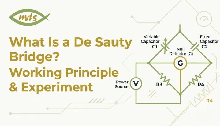
What Is a De Sauty bridge? Working Principle & Experiment

Posted on 21-07-202621-07-2026 by Tushar Saluja

TL;DR

This blog is for engineering students, electronics lab freshers, and anyone meeting bridge circuits for the first time, explaining De Sauty bridge in plain language before formulas show up.
A De Sauty bridge is a simple AC circuit used to compare an unknown capacitor against a known one, using a point where a headphone or detector goes silent as “answer.”
The core idea is balance, not complicated math. Once you understand why zero current in the detector arm means something useful, the whole circuit clicks.
De Sauty bridge experiment follows a repeatable procedure: set up four arms, apply an AC signal, adjust a resistor until you hit a null point, then calculate unknown capacitance from a simple ratio.
The bridge has one real weakness, dielectric loss in real world capacitors, and Grover’s modification exists specifically to fix it. Understanding that limitation is often exact thing exam questions test.

Also read,

Desauty bridge is a foundational AC bridge circuit used in electrical measurement to compare an unknown capacitor against a known standard capacitor. It remains a core part of electrical and electronics engineering lab curricula across Indian universities, both as a practical measurement method and as an introduction to balance principle used throughout instrumentation.

This guide explains how De Sauty bridge works, breaks down circuit and its components, and walks through De Sauty bridge experiment step by step, including observation table, calculation method, and common troubleshooting points. It also covers bridge’s key limitation with real capacitors, modifications introduced to address it, and where the same balancing principle continues to appear in current engineering research.

What Is a De Sauty bridge?

A De Sauty bridge is an AC bridge circuit used to measure or compare capacitance. In simple terms, it is a tool that tells you the value of an unknown capacitor by comparing it against a capacitor whose value you already know. It was developed by French engineer Paul de Sauty as one of earliest reliable methods for capacitor comparison, and it still shows up in electrical measurement labs across Indian engineering colleges today. The reason it has survived this long is simple: the circuit is easy to build, the math behind it is straightforward, and it teaches a concept that shows up everywhere in instrumentation, idea of balance.

Unlike a multimeter or a modern LCR meter that gives you a direct digital reading, a De Sauty bridge works by comparison. You adjust the circuit until it reaches a specific balanced state, and at that exact point, a simple ratio tells you unknown capacitance. It sounds old fashioned, and in some ways it is, but the underlying principle is the same one used inside far more advanced capacitance sensing systems today.

How a Bridge Circuit Actually Balances?

Before touching De Sauty bridge specifically, it helps to understand what a “bridge circuit” even means, because the word confuses a lot of first time learners.

Think of a bridge circuit as two parallel paths carrying the same electrical signal from a source to a detector. If both paths are perfectly matched, no difference in voltage appears between them, and a detector connected across the middle of two paths sees nothing, no current, no signal, no deflection. That state is called balance.

If two paths are not matched, there is a small voltage difference between them, and the detector picks it up. In older lab setups, that detector is often a pair of headphones connected through a small transformer, and instead of a needle moving, you literally hear a tone. As you adjust a resistor toward the correct value, tone gets quieter. At the exact balance point, sound disappears completely. That silent moment is called null deflection, and it is the entire trick behind how a De Sauty bridge works.

This matters because once you understand that balance simply means “both paths are now electrically identical,” the rest of the circuit stops feeling like memorized formulas and starts feeling like basic logic.

De Sauty bridge Circuit Diagram and Components

A De Sauty bridge has four arms arranged in a diamond or square shape, with an AC source connected across one diagonal and a detector connected across other diagonals.

Here is what typically sits in each arm:

Arm 1, contains an unknown capacitor, one whose value you are trying to find. Arm 2, contains a standard, known capacitor used as reference. Arm 3 and Arm 4, contain two non inductive resistors, meaning resistors built specifically so they do not behave like tiny inductors at AC frequencies. This matters because any stray inductance would throw off the balance condition.

An AC signal, usually from an audio oscillator around 1 kHz, is applied across one pair of opposite corners of this diamond. A detector, either a headphone based null detector or a digital null indicator in more modern trainer kits, is connected across other pairs of corners.

The basic idea is this: current splits and flows through both halves of the bridge at once, one half containing unknown capacitor and one resistor, the other half containing standard capacitor and other resistor. When the ratio of components on both sides matches perfectly, the detector arm carries zero current, and you have found your balance point.

De Sauty bridge Working Principle

Once physical layout makes sense, the working principle becomes much easier to follow.

De Sauty bridge works on principle of null deflection, which just means the circuit is adjusted until the detector shows no response at all. In an AC circuit, “no response” happens when electrical opposition, called impedance, on both halves of the bridge becomes proportionally equal. Impedance in this context is essentially resistance and capacitive effects combined, since capacitors do not behave like plain resistors under AC signals.

Balance Condition and Capacitance Formula

At balance, the impedance ratio across two arms is equal, which for this bridge simplifies into a very clean relationship between two capacitors and two resistors. Written simply, unknown capacitance equals standard capacitance multiplied by ratio of two resistor values.

Usually labeled R1 or R3 depending on the kit, balance condition gives:

C1 = C2 × (R4 / R3)

This is genuinely one of simplest formulas in electrical measurement, and that simplicity is exactly why De Sauty bridge is often the first bridge circuit taught to engineering students before more complex bridges like Maxwell’s or Schering’s bridge. You are not just learning one formula, you are learning a logic pattern that every other bridge circuit in your syllabus will reuse.

De Sauty bridge Experiment: Step by Step Procedure

This is part most lab manuals rush through, so here is the De Sauty bridge experiment broken down clearly, way it is typically performed on a standard trainer kit in a college lab.

Objective: To determine unknown capacitance of a capacitor using a De Sauty bridge.

Apparatus required: A De Sauty bridge trainer kit (with built in decade resistance dials and a standard capacitor), an audio frequency oscillator, a headphone or digital null detector, connecting wires, and unknown capacitor to be tested.

Procedure:

First, connect an unknown capacitor to the terminal marked for it on the trainer board. Next, connect the audio oscillator across the excitation terminals of the bridge, and connect the headphone or null detector across the detector terminals.

Switch on the oscillator. At this stage, you should hear a tone through headphones, or see a live reading on a digital null detector, confirming the bridge is receiving a signal but is not yet balanced.

Now slowly vary the resistance dial, usually labeled R1 or R3 depending on the kit, while listening carefully to headphone output, or watching detector reading. As you approach balance, tone will noticeably reduce in volume, or detector reading will drop toward zero.

Adjust carefully around this point until sound disappears entirely, or the detector shows minimum deflection. This is your null point. Note down resistance values at this exact setting.

Repeat this process at least three to five times, either by slightly disturbing and re-finding the balance point, or by testing with a different known standard capacitor value, to reduce impact of small human or instrument error.

Why De Sauty bridge Struggles with Real Capacitors

De Sauty bridge assumes every capacitor in circuit is a “pure” or ideal capacitor, one that only stores and releases energy without wasting any of it as heat.

Real capacitors are not perfectly ideal. Every practical capacitor has some internal energy loss caused by insulating material between its plates, called dielectric. This loss is known as dielectric loss, and it behaves almost like a hidden resistor sitting inside a capacitor.

Because the standard De Sauty bridge formula only accounts for pure capacitance and pure resistance, it cannot properly balance, or gives an inaccurate reading, when dielectric loss is significant. This is the single biggest limitation of basic De Sauty bridge, and it is almost guaranteed to come up as a viva question in your practical exam.

Grover’s Modified De Sauty bridge

To fix this dielectric loss problem, a modification was introduced, commonly credited to Grover, which adds two extra resistors into arms containing capacitors themselves.

These additional resistors are specifically placed to represent and account for internal loss inside each capacitor. With this change, a modified bridge can accurately measure both capacitance value and dissipation factor, a number that represents how “lossy” or imperfect a real capacitor actually is.

In practical terms, this modification turns De Sauty bridge from a circuit that only works on textbook perfect capacitors into one that can meaningfully test real components, which is exactly why modified versions appear in more advanced instrumentation labs and even in some published engineering research today.

Where De Sauty bridge Principle Shows Up Today

It is easy to assume a circuit this old is purely academic, something you learn for an exam and then forget. That is not entirely true.

The core balancing principle behind De Sauty bridge is still actively used in modern capacitive sensing research. Engineers working on structural health monitoring, practice of using sensors to detect tiny stress cracks or strain in bridges, buildings, and aircraft structures, have built wireless capacitive strain sensors around an analog De Sauty bridge design, precisely because balance based approach is sensitive enough to detect extremely small capacitance changes. Similar autobalancing versions of De Sauty bridge have also been explored for wide range capacitive sensor interfaces in wearable and biomedical devices, including experimental sensors designed to track tremor related signals.

This matters for you as a student because it reframes the entire lab experiment. You are not just learning a historical measurement trick, you are learning the exact same balance principle that underpins how many present day capacitive sensors are designed and calibrated. commercial LCR meters and digital bridge instruments used in modern electronics testing trace their conceptual roots directly back to bridge circuits like this one.

Advantages and Disadvantages of De Sauty bridge

De Sauty bridge earns its place in every basic electrical measurements syllabus for a few clear reasons, but it also comes with limitations worth knowing before your practical exam.

Advantages: circuit design is simple and inexpensive to build. The balance formula is easy to derive and calculate by hand. It offers good accuracy when measuring capacitors that are close to ideal, and it is an excellent teaching tool because it introduces the null deflection concept used throughout electrical instrumentation.

Disadvantages: basic version cannot accurately measure capacitors with meaningful dielectric loss, which covers a large share of real world capacitors. It requires a stable AC source and a sensitive detector to find a clean null point, and manually adjusting resistors to reach balance is slower than simply reading a value off a digital LCR meter.

Conclusion

De Sauty bridge is one of those rare topics that looks intimidating on paper but makes complete sense once you understand the single idea driving it, balance. Four arms, an AC signal, a detector listening for silence, and one clean formula connecting an unknown capacitor to a known one. That is the entire circuit, stripped of textbook language.

Running the De Sauty bridge experiment yourself is the fastest way to make this concept permanent rather than something memorized the night before an exam. Once you have physically turned that resistance dial, heard tone fade into silence, and calculated your first unknown capacitance from real observation data, bridge circuits as a whole, including more advanced ones waiting later in your syllabus, stop feeling like a wall of formulas and start feeling like a pattern you already understand. If you are heading into your electrical measurements lab this semester, keep this guide open beside your manual, and if a topic still feels unclear after your first attempt at experiment, that usually means it is worth revisiting once more before viva day rather than after.

FAQs

Q: What is the main use of a De Sauty bridge?

A De Sauty bridge is mainly used to measure or compare the value of an unknown capacitor against a known standard capacitor. It is a foundational instrument taught in electrical and electronics measurement labs to introduce the concept of AC bridge balancing.

Q: Why does De Sauty bridge use headphones as a detector?

Headphones are used because they are extremely sensitive to small AC signals at audio frequencies, making it easy for a student to hear the exact moment the bridge reaches null deflection. Some modern trainer kits replace headphones with a digital null detector for the same purpose.

Q: What is the formula used in the De Sauty bridge experiment?

At balance, unknown capacitance C1 equals standard capacitance C2 multiplied by the ratio of two resistors, written as C1 = C2 × (R4 / R3). This formula is derived directly from the impedance balance condition of the bridge.

Q: Why is De Sauty bridge considered inaccurate for real capacitors?

The basic De Sauty bridge assumes capacitors are ideal and lossless, but real capacitors have internal dielectric loss. This loss is not accounted for in the standard formula, which is why the bridge gives unreliable readings for capacitors with significant loss, unless a modified version is used.

Q: What is Grover's modification to De Sauty bridge?

Grover’s modification adds extra resistors into capacitor arms of the bridge specifically to account for dielectric loss. This allows modified De Sauty bridge to accurately measure both capacitance and dissipation factor of real, imperfect capacitors.

Q: Is De Sauty bridge still relevant in 2026?

Yes. While digital LCR meters have replaced it for routine industrial measurement, the underlying balance principle of De Sauty bridge is still used in current research areas like wireless structural health monitoring sensors and wide range capacitive sensor interfaces, making it more than just a historical lab exercise.

Tags: De Sauty bridge

What Is a Ballistic Galvanometer? Working Principle, Formula & Experiments

Posted on 07-07-202608-07-2026 by Tushar Saluja

TL;DR

This blog is for engineering and physics students, especially university freshers preparing for electromagnetism labs, who want a clear, beginner friendly explanation of what a ballistic galvanometer is and how it works.
A ballistic galvanometer does not measure current like a normal galvanometer. It measures total electric charge that passes through it in a short burst.
Its secret lies in two design choices: a heavy coil (large moment of inertia) and almost zero damping. Together, these let the first swing of the coil tell you exactly how much charge flowed.
key formula, Q = k × θ₀, connects charge Q to galvanometer constant k and first “throw” angle θ₀. Every lab experiment on this topic circles back to this one relationship.
Even though digital instruments have mostly replaced it in industry, ballistic galvanometers are still taught in Indian university labs because it builds a physical, hands-on understanding of charge, torque, and damping that a digital multimeter screen simply cannot teach.

Also read,

A ballistic galvanometer is a specialized instrument used to measure total quantity of electric charge that passes through a circuit during a brief, transient pulse, such as when a capacitor discharges. Unlike a standard galvanometer, which measures continuous current, a ballistic galvanometer is engineered to respond to a single short burst of charge and convert it into a measurable mechanical deflection.

This instrument remains a core component of undergraduate physics and electrical engineering laboratories, where it is used to determine charge, calibrate measurement constants, and calculate high resistance values through leakage methods. Its working principle rests on two deliberate design choices: a coil with a large moment of inertia and a suspension system with very low (minimal) damping. Together, these ensure that the coil’s first oscillation, known as first throw, is directly proportional to charge that passed through it.

This guide explains working principle, construction, formula, and standard laboratory experiments associated with ballistic galvanometers, along with its continued relevance in modern engineering education.

What Is a Ballistic Galvanometer, Really?

A regular galvanometer is designed to measure steady current by producing a deflection proportional to the current flowing through it. Give it a steady current, and its needle settles at a position that tells you how strong that current is.

A ballistic galvanometer has a very different job. It is a charge detective. Instead of measuring current flowing continuously, it measures the total amount of electric charge that passes through it during a brief pulse, like when a capacitor suddenly discharges.

Here is an important distinction that most textbooks gloss over: Current tells you the rate of charge flow, while a ballistic galvanometer measures the total charge that passes during a brief transient pulse. This is exactly like the swing example. It does not measure how long the current flows. Instead, it responds to the total charge transferred during the brief pulse, which is analogous to the total impulse delivered to the swing.

This makes a ballistic galvanometer, at its core, a charge measuring instrument, and this single idea is the foundation for everything else in this guide, including formula and experiments.

Why Does It Need Such a Heavy Coil?

If you have seen a ballistic galvanometer or read about its construction, you may have noticed something odd: The coil is deliberately made heavier and bulkier than in a normal galvanometer. This is not a manufacturing flaw. It is the entire trick behind how the device works.

Think about pushing two different swings, one that is very light and one that is heavy and solid. If you give both swings the exact same short, sharp push, the light swing will react almost instantly and start moving right away, even before you have finished pushing. heavy swing, on other hand, barely moves during push itself. It only really starts swinging after push is over.

That heavy swing is behaving like a ballistic galvanometer coil. Engineers deliberately increase the coil’s moment of inertia, which is just a technical way of saying “how much the coil resists changes in its rotational motion.” A heavy coil resists moving quickly, so by the time a brief charge pulse has finished passing through it, the coil has barely rotated at all. Only after the pulse is completely over does the coil start swinging freely, carrying with it the angular momentum imparted during the pulse.

This detail matters because it is what allows total charge, and not just a snapshot of current at one instant, to get “loaded” into coil’s motion before it starts moving.

Very Low Damping: The Other Half of the Trick

There’s another design option that makes this instrument possible and it’s as nifty as a heavy coil.

Suppose you are able to finally push that heavy swing and it begins to swing back and forth. Now envision a person standing beside it and gradually slowing it down each swing as it moves. Eventually the swing would stop, but of course there would be no clean means of determining how high the swing had been originally, since outside interference continued to take the energy of the swing.

In a normal galvanometer this is an “interference” which is actually useful. It’s known as damping and helps the needle settle rapidly without any oscillations. For a ballistic galvanometer damping is the enemy. When it swings and it loses energy to friction or electromagnetic braking, the very first swing will not be accurate in reflecting charge that passed through.

This is why a ballistic galvanometer is designed with very low (or minimal) damping. The coil is hung so that it is free to swing with as little air drag as possible and as little electromagnetic drag as possible. Therefore the first throw (first swing) occurs at an angle that is directly, and reliably proportional to the total charge that has passed through the coil.

A heavy coil and near zero damping is the distinguishing feature of a ballistic galvanometer from all other galvanometers, and is the one thing that most students recall from the ‘ballistic’ analogy as soon as they see it.

How First Throw Actually Happens: Step by Step

Now that you understand why coil is heavy and undamped, here is what physically happens when a charge pulse passes through it, laid out as a simple sequence:

Step 1: A brief pulse of charge, often from a discharging capacitor, flows through the coil.

Step 2: This charge experiences a force because the coil sits inside a strong magnetic field, produced by a permanent magnet. This is the same electromagnetic force that causes a current-carrying conductor in a magnetic field to experience torque.

Step 3: Because the pulse is so brief and the coil is so heavy, the coil does not move meaningfully during this force. Instead, the coil gains angular momentum while remaining almost stationary during the short current pulse, like a heavy object absorbing energy of a quick push.

Step 4: Once the pulse ends, the coil is now “loaded” with rotational energy, and it begins to swing freely, since there is almost no damping to interfere with it.

Step 5: coil swings to a maximum angle before a restoring force (usually from a suspension wire or spring) pulls it back. This maximum angle is first throw, θ₀.

Step 6: Because damping is negligible, this first throw angle is directly proportional to total charge that passed through the coil in Step 1.

This sequence is the physical story behind the formula you are about to see. Every symbol in that formula corresponds to one of these steps.

Ballistic Galvanometer Formula, Explained Term by Term

Once the coil absorbs the charge pulse and begins its first free swing, the relationship between charge and deflection can be derived using the physics of torque and angular momentum.

core working relationship is:

Q = k × θ₀

Where:

Q is total charge (in coulombs) that passed through coil
θ₀ is first throw, meaning maximum angle coil swings to on its very first oscillation
k is ballistic galvanometer constant, also called charge sensitivity constant

This proportional relationship is mathematically similar to other linear equations in physics, where one quantity is directly proportional to another through a constant. Like many proportional relationships in physics, charge is directly proportional to the first throw for a given instrument, which relates voltage, current and resistance. If the value of the constant k of that particular galvanometer is known, and the first throw angle is measured, then the exact charge passing through the galvanometer is known.

The value of constant k is related to the physical properties of the coil and a detailed derivation gives it in terms of the moment of inertia (I) of the coil, the magnetic field strength (B), the number of turns (N), the area (A) of the coil and the natural oscillation period (T) of the suspended coil. However, in the majority of undergraduate laboratories, you will not have to calculate k from first principles. Rather, you will measure it out, as the first experiment below shows.

There is also another concept related to it: current sensitivity, which describes the deflection of the coil for a steady current as compared to a one-time charge. This can be helpful for calibration but is a slightly different measurement to charge sensitivity used in the above formula.

Experiment 1: Measuring Charge on a Capacitor

This is a classic introductory experiment, and it is also how you calibrate a ballistic galvanometer before using it for anything else.

idea: You already know capacitance (C) of a capacitor and voltage (V) you charge it to. Using simple relationship Q = C × V, you can calculate the exact charge stored on the capacitor. Then, you discharge that capacitor through ballistic galvanometer and observe first throw angle θ₀. Since you now know both Q and θ₀, you can calculate k using Q = k × θ₀, and once k is known, galvanometer is calibrated for future experiments.

Simplified procedure:

The capacitor is connected to a known voltage source and allowed to charge fully. A switch is then flipped so the capacitor discharges through the galvanometer instead of voltage source. Because this discharge happens quickly, the coil experiences exactly the kind of brief, sharp pulse described earlier in this guide. coil swings to its first throw, θ₀, which is recorded, usually using a lamp and scale setup where a small mirror on coil reflects a beam of light onto a graduated scale, allowing very precise angle readings even for tiny deflections.

This procedure is repeated a few times to get a reliable average value of θ₀, and from there, ballistic constant k is calculated.

Why this experiment matters: It is not just a formality. This is literally how you find the k value that every other calculation in this guide depends on. Skipping careful calibration here is one of most common reasons student results in later experiments come out wrong.

Experiment 2: Measuring a High Resistance by Leakage Method

Once your galvanometer is calibrated, you can use it for more advanced measurements, and one classic application is determining an unknown high resistance, something that is genuinely difficult to measure directly with an ordinary ohmmeter.

Idea: A capacitor is first charged and discharged directly through galvanometer, giving an initial throw θ₀. This tells you charge when there is no extra resistance in the path. Next, the same capacitor is charged again, but this time it is allowed to slowly leak, or discharge, through unknown high resistance for a measured time, before finally being discharged through a galvanometer. Because some charge has already leaked away through resistance during that waiting period, second throw, θt, will be smaller than θ₀.

By comparing θ₀ and θt, and knowing capacitance and leakage time, unknown resistance can be calculated using:

R = t / [C × loge(θ₀ / θt)]

This formula might look intimidating, but conceptually it is simple. bigger resistance, slower leakage, and closer θt stays to θ₀. A smaller resistance lets charge escape faster, so θt drops more noticeably compared to θ₀.

Why this matters: This experiment is a great example of how ballistic galvanometer’s charge measuring ability can be repurposed to measure something else entirely, in this case, very high resistance values that are difficult to measure accurately using ordinary resistance measurement methods.

Advantages and Limitations You Should Know

Every instrument comes with trade-offs, and understanding them helps you appreciate why a ballistic galvanometer was designed the way it is, and why it eventually got replaced in most industrial settings.

Advantages:

scale is linear, meaning deflection is directly proportional to charge across its usable range, which makes calculations straightforward. It offers very high sensitivity, capable of detecting extremely small charge pulses. When properly shielded and calibrated, external magnetic field effects can be minimized, and its accuracy, when properly calibrated, is genuinely impressive for what is essentially a mechanical device.

Limitations:

Because it relies on springs, suspension wires, and a permanent magnet, it is prone to mechanical aging over time, meaning its calibration can drift and needs to be periodically rechecked. It is intended for measuring transient charge pulses, such as capacitor discharge currents, rather than continuous AC or steady-state current, since its entire principle depends on a brief pulse rather than continuous AC current. It is also inherently a manual, human read instrument, requiring careful observation of lamp and scale deflection, which introduces a small amount of human error compared to a digital readout.

Is the Ballistic Galvanometer Still Relevant in 2026?

It is a legitimate question and one student asks it. Why is this rather archaic mechanical device still in use today in Physics and Electrical Engineering?

The truth is, the ballistic galvanometer is hardly used in industrial and research applications anymore. Today, the measurement of charge is based on the integration of amplifiers, digital oscilloscopes and data acquisition systems that are faster, more precise and do not suffer from mechanical wear on springs or suspension wires. A special form of the ballistic galvanometer, the “fluxmeter,” was developed in the early 1900s to measure magnetic flux whose restoring torque was close to zero, and it has largely been replaced by electronic devices.

So why is it still included in the Indian University Physics lab course? Because it teaches something that a digital display cannot. As you observe the coil swing in a real experiment, observe the first throw and measure its maximum deflection, and then calculate the charge using Q = k × θ₀ to get an intuitive, physical understanding of concepts such as torque, angular momentum, and damping. This practical knowledge is what will arm engineering students when they study how modern digital sensors, oscilloscopes and measurement ICs function internally; they are all based on the same physics, but implemented electronically, not mechanically.

In other words, a ballistic galvanometer is less a tool you will use in your career and more a teaching instrument that helps you develop a physical intuition for every charge and current sensor you will meet later, whether it is a sensor in an EV battery management system, a precision agriculture sensor, or just a simple multimeter.

Wrapping It Up

A ballistic galvanometer is one of those instruments that looks intimidating on paper but makes complete sense once you connect it to something familiar, like a heavy swing absorbing a single sharp push. Its heavy coil and near zero damping work together so that its very first swing becomes a direct, reliable measure of total charge that passed through it, a relationship captured neatly in formula Q = k × θ₀. From calibrating a device using a known capacitor, to repurposing it for measuring high resistance through leakage method, this single principle of charge proportional deflection runs through everything the instrument is used for.

While digital instruments have taken over nearly every practical charge measurement task ballistic galvanometer once handled, it remains a fixture in Indian physics and electrical engineering labs precisely because it forces you to see and time a physical process, rather than simply reading a number off a screen. That hands-on intuition about torque, damping, and charge is exactly what makes concepts in modern electronics and sensor design click faster once you get there.

Frequently Asked Questions

What is the main difference between a ballistic galvanometer and a regular galvanometer?

A regular galvanometer measures continuous current and uses damping to settle its needle quickly. A ballistic galvanometer measures total charge from a brief pulse and is specifically designed with near zero damping so its first swing accurately reflects that charge.

Why is the coil of a ballistic galvanometer made heavier than usual?

A heavier coil has a larger moment of inertia, meaning it resists moving during a brief charge pulse itself. This ensures the coil absorbs the pulse’s energy first and only begins swinging afterward, which is essential for the first throw to correctly represent total charge.

What does the term "first throw" mean in a ballistic galvanometer experiment?

The first throw is maximum angle coil swings to on its very first oscillation after a charge pulse passes through it. Because damping is minimal, this angle is directly proportional to charge, as described by Q = k × θ₀.

Can a ballistic galvanometer measure AC current?

No. Its entire working principle depends on measuring total charge from a brief, transient pulse, similar to a capacitor discharge. It is not suited for continuous AC current measurement.

How is ballistic galvanometer constant k determined in practice?

It is typically found through a calibration experiment using a capacitor of known capacitance charged to a known voltage. Since charge Q = C × V is known, and first throw θ₀ is measured after discharging capacitor through galvanometer, k can be calculated using Q = k × θ₀.

Is ballistic galvanometer still used in real world engineering today?

Rarely in industry, since digital oscilloscopes and data acquisition systems have replaced it for practical charge and current measurement. However, it remains an important teaching instrument in Indian university labs because it builds a physical, intuitive understanding of charge, torque, and damping that underlies how modern digital sensors work.

Tags: ballistic galvanomete, ballistic galvanometer experiment

Carey Foster Bridge: Working Principle, Experiment & Applications

Posted on 07-07-202607-07-2026 by Tushar Saluja

TL;DR

This blog is for engineering students, university freshers, and physics lab learners in India who are studying the Carey Foster bridge experiment and want to actually understand it, not just memorize formulas for exams.
A Carey Foster bridge is a precision circuit built to measure very small or nearly equal resistances, something standard Wheatstone bridge struggles to do accurately.
The core trick is a slide wire and a clever “swap and re balance” step that cancels out errors from contact resistance and end connections automatically.
The balance condition formula looks intimidating at first, but it comes from the same null deflection logic as Wheatstone bridge, just applied twice.
This 1872 experiment is still on nearly every Indian engineering physics syllabus in 2026 because it builds measurement intuition that digital instruments hide from you.

If you have opened your first year engineering physics lab manual and spotted “Carey Foster Bridge Experiment” on the list, you are not alone in feeling a little lost. The name sounds complicated, the circuit diagram looks busy, and the formula involves symbols like l1, l2, P, Q, R, and S that seem to appear out of nowhere. This guide breaks the entire concept down from scratch, starting with what problem this bridge actually solves, before walking through circuit, experiment, and math behind carey foster bridge in plain, step by step language. By the end, you will understand not just how to perform the carey foster bridge experiment for your practical exam, but why it works and where this kind of precision measurement thinking still matters in 2026.

What Is a Carey Foster Bridge

Think about trying to compare the weight of two objects that are almost identical, say, two mobile phones from the same model. A regular kitchen scale will not help much here. It might show both as “180 grams” even if one is actually 2 grams heavier. To catch that tiny difference, you would need a much more sensitive balance, one built specifically to detect small differences rather than measure absolute weight. That is exactly the problem Carey Foster bridge solves, except with electrical resistance instead of weight. A Carey Foster bridge is an electrical circuit primarily used to measure low resistances and compare two nearly equal resistances with high precision. It was invented by British physicist George Carey Foster in 1872, as a modification of Wheatstone bridge, which was already a well known tool for resistance measurement at time. Foster introduced the modified bridge in 1872 in his paper On a Modified Form of Wheatstone’s Bridge, and Methods of Measuring Small Resistances. The keyword here is “modified.” Carey Foster bridge did not throw out the Wheatstone bridge concept and start fresh. It took the same null deflection principle and added one important component, a sliding wire, to fix a specific weakness. Understanding that weakness is the fastest way to understand why this bridge exists at all.

Why Wheatstone Bridge Falls Short

Before the slide wire trick makes sense, you need to know what a Wheatstone bridge actually does and where it struggles. A Wheatstone bridge works on a simple idea called null deflection. You arrange four resistances in a diamond shape, connect a battery across one diagonal and a galvanometer across another, and adjust one of the resistances until the galvanometer shows exactly zero current. At that exact balance point, a simple ratio relationship holds between four resistances, and you can calculate the unknown one using the other three known values. This works beautifully when you are measuring resistances in medium range, roughly a few ohms to a few thousand ohms, and when values you are comparing are reasonably different from each other. But it runs into trouble in two specific situations that matter a lot in real measurement work. First, when resistance you are measuring is very low, resistance of connecting wires and contacts themselves becomes large enough, relative to what you are measuring, to throw off the result. A wire’s own resistance, which is usually too small to matter, suddenly becomes a significant source of error. Second, when you are comparing two resistances that are almost identical, Wheatstone bridge’s sensitivity is not sharp enough to detect a small gap between them. Near-equal resistances produce only a very small change in the galvanometer reading around the balance point, making the exact null position harder to determine accurately. Carey Foster’s insight was that both problems could be solved with the same fix, a slide wire of uniform resistance placed between two of the bridge’s arms, combined with a simple swap and recheck measurement technique. That is the entire working principle of carey foster bridge in one sentence, and the next section unpacks exactly how it plays out in circuit.

Carey Foster Bridge Working Principle and Circuit

Picture Wheatstone bridge’s diamond shape, but with one important change. Instead of four fixed resistors sitting at four corners, Carey Foster bridge places a uniform slide wire, usually one metre long, stretched along a metre scale between two of its arms. A movable contact called a jockey can slide freely along this wire, and it connects to the galvanometer. The circuit has four resistance positions. Two of them, labelled P and Q, are known resistances chosen to be nearly equal to each other, often using a resistance box or two matched coils. The other two positions, X and Y, hold resistances you actually want to compare, one of which is usually a known standard and other unknown resistance you are trying to measure. At both ends of slide wire sit thick copper strips, sometimes called busbars, whose resistance is close enough to zero to be ignored. These copper strips exist purely to connect slide wire cleanly into the rest of the circuit without adding their own resistance into measurement. Here is where the null deflection principle from Wheatstone bridge comes back into play. You pass current through the circuit using a battery and a plug key, then slide jockey along wire until the galvanometer shows zero deflection, meaning no current flows through it. At that exact point, the bridge is balanced, and the same ratio logic that governs a Wheatstone bridge applies here too. But Carey Foster bridge does not stop at one balance reading. It takes a second reading after swapping positions of X and Y, and this second step is where real precision comes from. The next section explains exactly why this swap matters so much.

Carey Foster Bridge Experiment Step by Step

If you are heading into the lab for this practical, here is a procedure laid out in order you will actually perform it, along with what is happening physically at each stage. You begin by setting up apparatus: Carey Foster bridge itself with its metre long slide wire, a resistance box, a galvanometer, a battery with a plug key, a thick copper strip, connecting wires, Repeat this process, this time replacing copper strip with your unknown resistance wire to measure that wire’s diameter. Start by connecting known resistances P and Q on either side such that their ratio is close to one, meaning P and Q should be nearly equal. This keeps the bridge sensitive across the full length of slide wire rather than bunching all sensitivity near one end. The experiment is normally performed in two stages. First, a known standard resistance is used to determine the resistance per unit length (σ) of the slide wire. After this calibration, the known standard is replaced with the unknown resistance, and the balancing procedure is repeated to determine its value. Now comes the defining move of this experiment. Swap positions of copper strip and known resistance, so whichever gap had copper strip now has resistance, and vice versa. Slide jockey again to find a new null point, and note this position as l2. distance between l1 and l2 corresponds directly to resistance per unit length of slide wire, once you know the value of resistance you used. Repeat this process, this time replacing copper strip with your unknown resistance wire in place of known resistance box value, to find unknown resistance itself using the same swap and balance method. Finally, measure length and diameter of unknown wire using a metre scale and screw gauge, since these values feed into calculating specific resistance, also called resistivity, of wire’s material.

Understanding End Correction

This is part of the Carey foster bridge experiment that trips up most students, not because the concept is hard, but because textbooks usually explain it using only symbols. Here it is in plain language first. When you connect a resistance into one of the gaps of a bridge, that connection is not perfectly resistance free. metal strips, screws, and contact points at each end of slide wire add a tiny bit of extra, unwanted resistance that gets mixed into your reading. This unwanted extra resistance is called end resistance or end correction, and if left unaccounted for, it quietly throws off your final answer. Here is an elegant part of Carey Foster’s design. That end resistance error exists whether you measure copper strip position or resistance box position, and crucially, it exists in the same way both times. So when you take a second reading after swapping X and Y, the end correction error appears identically in both readings. When you then look at the difference between l2 and l1 rather than either value on its own, that shared error cancels itself out completely. You never need to measure or calculate end resistance separately. The swap and subtract method handles it automatically, which is precisely why Carey Foster bridge is so much better at low resistance and near equal resistance measurements than a plain Wheatstone bridge. This is genuinely one of more beautiful pieces of measurement design in classical electrical experiments. Instead of trying to eliminate an error directly, Foster designed a procedure where error cancels itself through subtraction.

Balance Condition and Formula Derivation

Now that swap logic makes intuitive sense, the formula itself becomes much easier to follow. It comes directly from applying Wheatstone bridge balance condition twice and comparing two results. In a standard Wheatstone bridge, the balance condition is P/Q = R/S, meaning the ratio of one pair of arms equals the ratio of the other pair at the null point. In Carey Foster bridge, “R” and “S” arms are effectively X plus a length of slide wire, and Y plus remaining length of slide wire. If sigma (σ) represents resistance per unit length of slide wire, and l1 is the first balance point measured from the left end, the balance condition for first reading works out to a relationship between P, Q, X, Y, l1, and σ. When you swap X and Y and take a second reading at l2, you get a second equation with the same structure, just with X and Y exchanged and l1 replaced by l2. Because P and Q, and underlying physical setup, stay exactly the same between both readings, two equations share the same left hand side. That means their right hand sides must be equal too. When you set them equal and simplify algebraically, most of terms cancel out, leaving a strikingly simple final relationship: X minus Y equals σ multiplied by (l2 minus l1) In words, the difference between two resistances X and Y is simply equal to the resistance of the length of slide wire lying between two balance points. This is a balance condition formula that every carey foster bridge experiment lab manual will ask you to derive and apply. Once you know σ, resistance per unit length of wire, you can find any unknown resistance by measuring balancing lengths before and after swapping. And once you know unknown wire’s resistance, its specific resistance, or resistivity, can be calculated using standard formula R equals rho L divided by pi r squared, where L is wire’s length and r is its radius from screw gauge measurement.

Carey Foster Bridge vs Wheatstone Bridge vs Kelvin Bridge

Since exam questions and viva sessions often ask students to distinguish between these three, here is a clear side by side comparison.

Feature	Wheatstone Bridge	Carey Foster Bridge	Kelvin Double Bridge
Best suited for	Moderate resistance measurements	Low resistances and near equal resistance comparison	Very low resistances (typically below 1 ohm)
Key structural feature	Four fixed resistance arms	Slide wire inserted between two arms	Second set of ratio arms to cancel lead and contact resistance
Handles contact/end resistance error	No, this limits its precision at low values	Yes, cancelled automatically via swap method	Yes, cancelled through double ratio arm design
Typical use case	General lab resistance measurement, strain gauge circuits	Comparing nearly identical resistances, finding specific resistance of wires	Measuring resistance of cables, contacts, and connectors

Three bridges are best understood as a family, not rivals. Carey Foster bridge is essentially a specialized, higher precision form of Wheatstone bridge, while Kelvin Double Bridge takes concept further still, specifically engineered to eliminate effect of contact and lead resistances when measuring very low resistances. Each one exists because the previous design had a specific blind spot that engineers needed to close.

Advantages, Limitations, and Precautions

Like any measurement tool, Carey Foster bridge has strengths worth appreciating and limitations worth knowing before your practical exam or viva. On the advantage side, this bridge delivers genuinely high precision for the specific job it is designed for. Because measurements are based on locating a null point rather than estimating a scale reading, observational errors are reduced. swap and subtract method eliminates end correction and contact resistance errors without any extra calculation. The apparatus itself is also low cost and low maintenance, since it uses simple components like a slide wire, a galvanometer, and a resistance box, all of which are widely available in college labs across India. On the limitation side, slide wire needs periodic calibration, since repeated sliding of jockey contact can wear down wire’s surface over time and change its resistance per unit length slightly. The bridge is also sensitive to temperature, since resistance of both slide wire and wire being tested can shift if the room heats up during a long measurement session. It is a manual, DC only method, meaning it is not suited for AC resistance or impedance measurements, and it takes noticeably longer to perform than simply plugging a wire into a digital multimeter. A few precautions make a real difference to your results. Keep the balance point confined to the middle third of slide wire whenever possible, since sensitivity is highest there and lowest near ends. Never let jockey drag along wire, press it down briefly at each test point instead, since dragging scratches wire and changes its resistance over time. Always include a plug key in the battery circuit and only close it briefly while taking readings, since prolonged current flow heats wire and drifts your balance point. Keep P and Q resistances genuinely close in value, since a large mismatch between them reduces bridge’s overall sensitivity.

Real World Applications in 2026

It is fair to ask why a 150 year old measurement technique still matters when digital micro ohmmeters and four wire Kelvin measurement systems can give you a resistance reading almost instantly. The honest answer has two parts, one practical and one educational. On the practical side, underlying null deflection and swap cancellation principles behind Carey Foster bridge are still embedded in how precision resistance and strain measurement instruments are designed today, even when the interface is now a digital display instead of a galvanometer needle. Modern four-wire Kelvin sensing addresses the same measurement challenge reducing errors caused by lead and contact resistance but does so using a different electrical approach. this using separate current and voltage paths, the Carey Foster Bridge reaches a similar goal through its swap-and-balance method to cancel out contact and lead resistance errors, exactly what Foster’s swap method achieved with a slide wire in 1872. The bridge circuit family this experiment belongs to also continues to matter directly in fields like strain gauge measurement, where sensors used in load cells, pressure sensors, and structural health monitoring systems still rely on bridge configurations to detect tiny resistance changes with high sensitivity. On educational side, and this is part most students underestimate, carey foster bridge experiment remains on nearly every Indian engineering physics syllabus, from AKTU to BIT Mesra to Delhi University affiliated colleges, precisely because it forces you to understand where measurement error comes from and how deliberate procedure design eliminates it. A digital multimeter hides all of this from you. You press a button and get a number, with no insight into contact resistance, end correction, or sensitivity trade offs. This experiment builds an intuition for precision measurement that becomes genuinely valuable the moment you step into any lab, quality control floor, or calibration facility in your career. Several Indian institutes now provide access to Virtual Labs simulations that allow students to practice the Carey Foster Bridge experiment before or alongside physical laboratory sessions., allowing students to perform simulated Carey Foster Bridge experiments online before or alongside physical laboratory sessions, now also offer simulated versions of this experiment online, letting students practice balancing and swapping procedure digitally before or alongside physical lab sessions, a genuinely useful 2026 era addition to how this century old experiment is taught.

Why This Experiment Still Matters: Career Pathways for Indian Engineering Students

If you are doing this experiment as part of your first year B.Tech or B.E. physics lab, it is worth connecting it to where this kind of thinking leads professionally, because precision measurement is a real, well paying career track in India, not just a lab exercise you forget after the exam. Students who genuinely enjoy logic behind bridge circuits, error cancellation, and precision measurement often find a natural fit in instrumentation and control engineering, a specialization offered as a dedicated B.Tech branch or as electronics and instrumentation engineering at institutes across the country. This field centers on science and technology of measurement and control, spanning sensors, transducers, control systems, automation, electronics, and signal processing, all of which trace their conceptual roots back to exactly the kind of null deflection Carey Foster bridge teaches. career outcomes are genuinely solid for students entering this space. In 2026, instrumentation graduates increasingly work as specialists who design and manage sensor networks and control systems powering automated factories, smart cities, and sustainable energy plants, roles that barely existed in this form a decade ago. Entry-level instrumentation engineers can find opportunities across manufacturing, energy, automation, and process industries, with salaries varying widely by employer, location, and qualifications that vary by employer, location, and qualifications, with experienced professionals earning substantially more as they move into specialized roles. Government and public sector opportunities are also significant in this space. Public sector undertakings including ONGC, BHEL, and SAIL regularly hire instrumentation engineers, typically through GATE qualified recruitment, making this one of more stable long term career routes available to engineering graduates who build a strong foundation in measurement principles early on. Beyond core instrumentation roles, this foundational understanding of precision measurement also feeds naturally into calibration laboratories, quality control departments in manufacturing, semiconductor testing facilities, and research roles in national physical science institutions, all of which value engineers who understand measurement error at a conceptual level rather than only knowing how to read a digital display.

Conclusion

The Carey Foster bridge experiment can feel like just another entry on a long physics practical list, but thinking behind it is genuinely elegant once broken down step by step. It takes familiar null deflection logic of Wheatstone bridge and adds a slide wire and a simple swap procedure that automatically cancels out end correction and contact resistance errors, letting it measure low and near equal resistances with a precision original Wheatstone design could never achieve on its own. Understanding why each step of procedure exists, rather than memorizing formula X minus Y equals sigma times l2 minus l1 in isolation, is what will actually help you in your viva, your practical exam, and any future work involving precision instrumentation. This 1872 invention still earns its place on Indian engineering syllabi in 2026 because the core idea behind it, cancelling systematic error through careful procedural design rather than expensive equipment, remains exactly how modern precision measurement instruments are engineered today. Next time you are in the lab sliding that jockey contact along wire, you are practicing a measurement philosophy that genuinely carries through into real instrumentation and metrology careers.

FAQs

What is the main purpose of Carey Foster bridge?

Carey Foster bridge is primarily used to measure very low resistances and to compare two nearly equal resistances with high precision, a task where a standard Wheatstone bridge is not accurate enough due to end correction and contact resistance errors.

Why do we interchange resistances in the Carey Foster bridge experiment?

Interchanging or swapping positions of two resistances being compared causes unwanted end resistance error to appear identically in both balance readings. When you subtract two readings to find difference, this shared error cancels out automatically, which is the central working principle of carey foster bridge.

What is the formula used in the Carey Foster bridge experiment?

The balance condition formula is X minus Y = σ(l2 minus l1), where X and Y are two resistances being compared, σ is resistance per unit length of slide wire, and l1 and l2 are balance point positions before and after swapping X and Y.

How is Carey Foster bridge different from Wheatstone bridge?

Wheatstone bridge uses four fixed resistance arms and works well for general medium resistance measurement, while Carey Foster bridge adds a slide wire between two arms and uses a swap and balance procedure specifically to achieve higher precision for low resistances and near equal comparisons.

Why is this experiment still taught in Indian engineering colleges in 2026?

Even though digital resistance meters exist, this experiment builds a hands-on understanding of measurement error, end correction, and precision procedure design that digital instruments hide behind a simple numeric display, making it valuable groundwork for instrumentation, metrology, and quality engineering careers.

What precautions should be taken during the Carey Foster bridge experiment?

Keep balance point in middle portion of slide wire for best sensitivity, avoid dragging jockey along wire to prevent scratching it, keep plug key closed only briefly while taking readings to avoid heating effects, and ensure P and Q resistances used are genuinely close in value.

Tags: carey foster bridge experiment

SOC and SOH in BMS: Understanding Battery State Estimation in Electric Vehicles

Posted on 01-07-202601-07-2026 by Tushar Saluja

TL;DR

This blog is for engineering students, EV enthusiasts, and freshers in India who want to understand SOC and SOH in BMS, what these parameters mean, how a Battery Management System estimates them, and why accurate estimation is critical for safe and efficient EV operation.
SOC (State of Charge) tells you how much energy is left in the battery right now, like a fuel gauge. SOH (State of Health) tells you how much total capacity the battery still has compared to when it was new.
Estimating SOC and SOH in a battery is far harder than it looks; these values cannot be measured directly and must be calculated using algorithms that combine voltage, current, and temperature data in real time.
Modern BMS systems use a progression of methods from simple Coulomb Counting to Extended Kalman Filters and AI-driven machine learning models, each improving on accuracy and adaptability but requiring more computational power.
SOC and SOH algorithm development is one of most technically demanding and high-paying BMS specializations in India’s EV sector.

There is a single number displayed on every electric vehicle dashboard that drivers check more anxiously than anything else: battery percentage. That reading is not a direct measurement. BMS cannot stick a probe into a battery cell and read the remaining energy way you measure liquid in a tank. Instead, it estimates figures continuously using a combination of sensor data, electrochemical models, and sophisticated algorithms. Getting this estimation wrong has real consequences for drivers, for battery longevity, and for safety.

SOC and SOH in BMS are two most important state parameters that every Battery Management System must continuously compute and communicate. SOC in BMS is a real-time energy gauge. SOH is a long-term health metric. Together, accuracy of their estimation determines whether an EV can maximize its range, protect its battery from harmful conditions, and give drivers reliable information to make decisions. This blog explains both concepts from the ground up, walks through how modern BMS systems estimate them, and connects this technical knowledge to practical career opportunities in India’s fast-growing EV industry.

What Is SOC in BMS? Real-Time Energy Gauge

Think about the fuel gauge in a conventional petrol car. When the tank is full, it reads 100%. When it is empty, it reads 0%. gauge directly reflects the amount of fuel remaining. The state of Charge in a battery works on the same intuitive principle, but the physics underneath are fundamentally different.

SOC is defined as the ratio of the battery’s remaining available charge to its current usable capacity, expressed as a percentage, expressed as a percentage. A battery at 75% SOC has three-quarters of its usable energy remaining. A battery at 20% SOC is approaching a lower protection limit enforced by BMS to prevent deep discharge damage.

The critical word here is “estimate.” Unlike a fuel tank where you can measure liquid volume directly, a battery’s stored energy is locked inside an electrochemical system. There is no sensor that can directly read SOC. BMS must infer it indirectly by measuring external observable parameters it can access primarily voltage, current, and temperature and computing SOC from them using algorithms.

This estimation challenge is what makes SOC in BMS a genuinely difficult engineering problem. Battery voltage does have a relationship with SOC; a fuller battery sits at higher voltage but this relationship is highly non-linear, temperature-dependent, and shifts as battery ages. BMS must account for all these variables simultaneously, in real time, across every driving and charging scenario, Production EV BMSs generally aim for SOC estimation errors within a few percentage points under normal operating conditions of true value.

Why does accuracy matter this much? An overestimated SOC reading might let a driver attempt a trip that battery cannot actually complete, leading to a stranded vehicle. An underestimated SOC might trigger an early protective cutoff, wasting usable range. And an inaccurate SOC reading misleads BMS’s own internal algorithms for cell balancing, charging management, and protection logic creating a cascade of errors across the entire battery control system.

What Is SOH in BMS? Long-Term Health Metric

If SOC answers the question “how much energy is left right now,” then SOH answers an equally important question: “how much energy can this battery hold at all, compared to when it was new?”

State of Health is defined as ratio of battery’s current maximum capacity to its original rated capacity when new, expressed as a percentage. A battery with 85% SOH can hold 85% of energy it could store on the day it left the factory. The remaining 15% has been permanently lost to gradual degradation processes such as lithium inventory loss, electrode aging, and SEI layer growth.

industry-standard end-of-first-life threshold for an EV battery is 80% SOH. This is the point at which accumulated capacity loss becomes noticeable enough to significantly affect real-world driving range. It is also standard against which EV battery warranties in India are typically measured. Most manufacturers guarantee that their battery will retain at least 70 to 80% SOH for 8 years or a specified mileage.

SOH can be expressed through two lenses. capacity-based SOH compares current maximum charge capacity against original rated capacity in ampere-hours. This is the most common definition used by manufacturers and service engineers. Resistance-based SOH tracks the battery’s internal resistance, which increases as battery ages due to thickening of the SEI layer on anode, electrolyte decomposition, and electrode material degradation. Rising internal resistance reduces the battery’s ability to deliver high currents cleanly, causing voltage to sag under load and peak power to diminish even if capacity has not fallen as dramatically.

Both lenses together give engineers a complete picture of battery aging. Capacity fade tells you how much energy storage has been lost. Resistance increase tells you how much power delivery capability has been compromised. In a well-designed BMS, SOH monitoring tracks both.

Why SOC and SOH Are Coupled and Why That Makes Estimation Harder

One of the subtler challenges in BMS design is that SOC and SOH in a battery are not independent. They influence each other in ways that complicate accurate estimation of either.

Consider what happens as a battery ages and its SOH declines. The battery’s true maximum capacity is now lower than rated value. If BMS is still using original rated capacity to calculate SOC, its SOC estimates will drift away from reality. A battery with 80% SOH that is fully charged only holds 80% of its original energy capacity. If the BMS continues using the original rated capacity instead of the updated degraded capacity in its SOC calculations, SOC estimates can become inaccurate and drift from the battery’s true usable state.

Conversely, an outdated SOH figure causes errors in the SOC algorithm. When a BMS knows that a battery’s actual capacity has degraded, it must update the denominator used in SOC calculation accordingly. This is why modern BMS systems run SOC and SOH estimation algorithms jointly, feeding each other’s outputs as inputs. Accurate SOH feeds into SOC algorithm to keep fuel gauge accurate over battery’s life. And accurate SOC history feeds into SOH algorithms to identify capacity fade trends over hundreds of cycles.

This coupling is also relevant for range estimation. The driving range EV dashboard displays are not computed from SOC alone.It is estimated using remaining battery energy (which depends on both SOC and SOH) together with predicted energy consumption, driving conditions, and vehicle efficiency models. A degraded battery with poor SOH displays both a shorter maximum range and a faster-falling SOC percentage as it discharges, which can feel surprising to owners who do not understand connection.

How BMS Estimates SOC in a Battery From Simple to Sophisticated

The engineering challenge of estimating SOC in BMS has produced a range of methods, each with different trade-offs between simplicity, accuracy, computational cost, and robustness to real-world conditions.

Coulomb Counting Foundational Method

Coulomb Counting is the simplest and most widely used baseline method for SOC estimation. The principle is elegant: if you know how much charge went into the battery during charging and how much has come out during discharging, you can calculate remaining SOC by tracking net cumulative current over time.

In practice, BMS uses a current sensor to measure current flowing in and out of the battery pack every few milliseconds. It integrates this current over time (multiplied by efficiency factors) to update SOC figures continuously. The method is computationally simple, requires no battery model, and works in real time.

The weakness of Coulomb Counting is error accumulation. Current sensors have small measurement errors, and these errors integrate over time along with current itself causing SOC estimates to drift away from true value across a full charge-discharge cycle. The method also requires an accurate initial SOC to start from, and it has no self-correcting mechanism to compensate for accumulated drift. In a real vehicle that is charged and driven daily, uncorrected Coulomb Counting can produce SOC errors of 5 to 10% after a few weeks of operation.

Most BMS implementations use Coulomb Counting as primary real-time tracking method but combine it with a correction step based on voltage measurements when the battery is at rest.

Open Circuit Voltage Method Calibration Anchor

When a lithium-ion battery has been at rest for a sufficient period with no current flowing, it reaches electrochemical equilibrium and its terminal voltage stabilizes at Open Circuit Voltage (OCV). This OCV has a well-characterized relationship with SOC; each chemistry (NMC, LFP, NCA) has its own OCV-SOC curve established through laboratory testing.

By measuring OCV when a vehicle has been parked for long enough, BMS can look up corresponding SOC directly from this curve and use it to reset the Coulomb Counting accumulator, correcting any drift that has built up since last calibration.

The limitation is practical: OCV method only works when the battery is truly at rest, which does not happen during driving or active charging. It also requires vehicles to be parked for some time typically 30 minutes to several hours depending on chemistry before voltage fully stabilizes. LFP batteries present a particular challenge here because their OCV-SOC curve is very flat across a wide range of SOC, meaning small voltage measurement errors translate to large SOC errors during OCV-based calibration.

Extended Kalman Filter Adaptive Estimator

Extended Kalman Filter, or EKF, is the most widely deployed advanced SOC estimation method in production EV Battery Management Systems. It addresses limitations of both Coulomb Counting and OCV methods by combining their strengths within a mathematical framework that handles noise, uncertainty, and non-linearity.

Kalman Filter is fundamentally a recursive estimation algorithm. It maintains an internal model of the battery , typically an equivalent circuit model that represents the battery’s electrical behavior using resistors and capacitors and runs a continuous prediction-and-correction loop. At each step, it predicts what battery voltage should be based on its current SOC estimate and equivalent circuit model. Then it compares that prediction against actual measured voltage. The difference between the two is “innovation” , new information that updates SOC estimates.

“extended” version handles non-linear relationships between battery voltage and SOC that plain Kalman filters cannot manage, using linearization techniques at each update step. The result is an estimator that is robust to measurement noise, self-correcting against accumulated Coulomb Counting drift, and capable of tracking SOC accurately even through dynamic driving conditions, hard acceleration, regenerative braking, varying temperatures.

EKF can converge, EKF can converge toward an accurate SOC estimate even when the initial SOC estimate is significantly incorrect. EKF can converge toward an accurate SOC estimate even when the initial estimate is significantly incorrect. This robustness to initial conditions is critical for vehicles that have been parked for an extended time or in conditions where no OCV rest measurement was possible.

Machine Learning and AI-Based Methods Next Frontier

As EV fleets have grown and battery datasets have become richer, data-driven approaches using machine learning have entered BMS design for SOC and SOH estimation. Methods including LSTM (Long Short-Term Memory) neural networks, Gaussian Process Regression, and hybrid models that combine physics-based algorithms with ML layers are 97% accuracy in several published research studies in research settings.

The advantage of ML-based methods is their ability to capture complex, non-linear patterns in battery behavior that analytical models approximate imperfectly including subtle effects of battery aging, temperature variation, and chemistry-specific quirks. A well-trained LSTM network can learn from millions of charge-discharge cycles across a fleet of vehicles, effectively building an empirical model of battery behavior that improves over time with more data.

The challenge is computational: neural networks require more processing power than Kalman filters, which can strain microcontrollers embedded in BMS hardware. This has driven research into hybrid architectures using lighter ML models to correct or adapt classical filter-based estimators rather than replacing them entirely. Hybrid AI approaches combining physics-based models with ML layers have demonstrated SOH estimation accuracies approaching 97%, making them increasingly practical for production systems where OTA (Over-the-Air) updates can push improved algorithm versions to vehicles already in the field.

Several automotive engineering firms, including Tata Elxsi, have publicly highlighted work on advanced BMS platforms that incorporate improved SOC and SOH estimation capabilities for EV applications alongside conventional sensor monitoring, enabling more accurate range prediction and longer-term battery health tracking under Indian operating conditions.

How BMS Estimates SOH in a Battery

SOH estimation is fundamentally different from SOC estimation in one important way: SOH changes slowly over months and years, not moment to moment. This means algorithms tracking it operate on longer time scales and use different signals.

Capacity-Based SOH Estimation

The most direct approach to measuring SOH is to periodically perform a full charge-discharge cycle under controlled conditions and measure how much charge the battery actually accepts and delivers. Comparing this measured capacity to original rated capacity gives capacity-based SOH.

In a real EV, performing a full controlled cycle just to measure capacity is impractical. Instead, BMS systems reconstruct equivalent information from daily driving and charging data. When a vehicle is charged from a known low SOC to a known high SOC, BMS integrates current flow to measure how much charge was actually delivered and compares this to what original battery specifications would predict for the same SOC window. Doing this repeatedly across many charging sessions builds a statistical picture of how the battery’s actual capacity is changing over time.

Internal Resistance Tracking

Alongside capacity fade, rising internal resistance is another primary indicator of battery aging and a key input to resistance-based SOH estimation. As a battery ages through SEI layer growth, electrode degradation, and electrolyte decomposition, its internal resistance climbs. This shows up as increasing voltage drop under high-current loads, reduced peak power delivery, and greater heat generation during charging and discharging.

BMS tracks internal resistance through electrochemical impedance analysis applying a known current pulse and measuring immediate voltage response and through more sophisticated electrochemical impedance analysis in advanced systems. Comparing present internal resistance to beginning-of-life internal resistance gives a health indicator that complements capacity-based SOH and is particularly useful for detecting power fade in batteries that have not yet lost much total capacity.

Adaptive and AI-Driven SOH Estimation

Because SOH evolves slowly and depends on accumulated usage history, machine learning approaches are especially well-suited to SOH estimation. AI models trained on large battery aging datasets can learn to predict current and future SOH from patterns in voltage, temperature, and current data that develop subtly over hundreds of cycles.

Research combining machine learning with physics-based aging indicators has demonstrated SOH estimation accuracy above 97% on real-world battery datasets. growing availability of cloud-connected BMS systems where vehicle telemetry data from thousands of cars feeds into centralized machine learning models is accelerating this capability. Fleet-level SOH modeling enables manufacturers to predict battery replacement needs ahead of failure, optimize warranty management, and identify chemistry or usage patterns that accelerate aging in specific geographic or climatic conditions.

SOC and SOH Estimation in Indian EVs Real-World Context

India’s unique operating conditions create specific challenges for SOC and SOH estimation that are not fully addressed by algorithms developed for European or North American climates.

Battery voltage and OCV-SOC relationship are both temperature-dependent, and India’s wide temperature range from sub-zero winters in Himalayas to 48-degree Celsius summers in Rajasthan and Gujarat means BMS algorithms must be robustly calibrated across a far wider thermal envelope than temperate-climate markets require. An OCV-SOC lookup table calibrated at 25 degrees Celsius introduces SOC estimation errors when used at 45 degrees. Algorithms that correctly compensate for temperature across the full Indian range are a genuine engineering differentiator.

Ather 450X is an example of an Indian EV where SOC accuracy has been emphasized as a feature. Ather Energy’s BMS provides highly granular real-time battery state data to riders through its connected dashboard and companion app, with software and thermal management working together to improve battery monitoring and estimation accuracy by keeping cells within a well-characterized temperature range. Real-world incidents involving inaccurate range estimation have highlighted why SOC estimation accuracy is critical. In connected EV platforms, OTA firmware updates can improve estimation algorithms without requiring hardware changes demonstrating advantage of connected, updatable BMS software architectures.

Tata Motors and Tata Elxsi have collaborated on EV software and battery-management technologies, including work related to battery monitoring, battery-management software, and connected EV technologies, which integrates SOC and SOH estimation with OTA update capability. OTA-capable EV platforms make it possible for manufacturers to improve battery-management software over time through firmware updates where supported, refined through accumulated fleet data and algorithm improvements pushed wirelessly to all vehicles.

LFP chemistry, dominant in Indian EVs, presents a specific SOC estimation challenge due to its flat OCV-SOC curve. In NMC batteries, voltage changes significantly with SOC, giving OCV-based correction methods a clear signal to work with. In LFP, OCV changes by only about 0.1 volts across a wide mid-SOC range, making it very difficult to calibrate SOC accurately from voltage alone. LFP BMS designs therefore rely more heavily on Coulomb Counting accuracy and on Kalman Filter-type algorithms that can extract SOC from subtle dynamics of voltage response rather than from static OCV level.

Why SOC and SOH Estimation Is Technically Difficult

It is worth pausing to appreciate why SOC and SOH estimation in BMS systems is a genuinely hard engineering problem, not a straightforward measurement task.

The core difficulty is that quantities of interest stored energy and battery health are internal states of an electrochemical system that can only be inferred from external measurements. Voltage, current, and temperature are only signals available. Yet each of these measurements is imperfect: current sensors have noise and drift, temperature sensors may not reflect actual cell-core temperature, and voltage is a function of both SOC and internal resistance (which itself changes with temperature, aging, and current history in complex ways).

Battery behavior is also highly non-linear. The same voltage reading might correspond to different SOC values depending on whether the battery is charging or discharging (hysteresis), recent current history (relaxation effects), temperature, and battery’s age. These non-linearities must all be modeled and accounted for in the estimation algorithm.

And unlike most engineering systems, batteries change their fundamental characteristics over time as they age. An algorithm perfectly calibrated for a new battery becomes progressively less accurate as the same battery ages, which is why SOC and SOH estimation must be adaptive, continuously updating its internal model parameters to match the battery’s changing behavior.

This combination of unmeasured internal states, imperfect sensors, non-linear behavior, and time-varying characteristics is what makes SOC and SOH in battery systems a rich area for both academic research and practical engineering innovation.

Career Opportunities in SOC and SOH Algorithm Development for Students

For engineering students in India, SOC and SOH estimation represents one of most technically sophisticated and highly compensated specializations within BMS engineering domain.

BMS Algorithm Engineers who develop SOC and SOH estimation algorithms are among the most sought-after technical roles in India’s EV ecosystem. Companies including Tata Elxsi, Ather Energy, Ola Electric, Ultraviolette Automotive, Log9 Materials, Mahindra Electric, and Bosch India are actively building BMS software teams and recruiting engineers with estimation algorithm expertise. Ultraviolette Automotive explicitly lists algorithm development for SOC, SOH, and SOP (State of Power) estimation as a core responsibility in its BMS engineer job descriptions, alongside testing with hardware-in-the-loop (HIL) systems and compliance with AIS and ISO safety standards.

technical skills that employers in this space look for span several disciplines. Strong mathematical foundations in estimation theory understanding Kalman Filters, state-space models, and basics of system identification are essential. MATLAB and Simulink proficiency is expected for algorithm prototyping and model-based development, with embedded C or Python required for translating algorithms into BMS firmware. Electrochemistry fundamentals help engineers build better equivalent circuit models and understand why their algorithms behave the way they do in real cells. Knowledge of automotive communication protocols like CAN bus is needed for integrating BMS algorithms with vehicle-level systems.

Machine learning expertise is becoming increasingly valuable in this space. Engineers who can combine classical Kalman Filter methods with LSTM networks or Gaussian Process Regression models, and who understand how to validate and deploy these on embedded hardware with limited computational resources, represent a genuinely scarce profile with strong salary premiums. According to industry data, Engineers with expertise in SOC/SOH estimation, battery modeling, and control algorithms are generally considered among the more specialized BMS professionals, often commanding competitive salaries depending on their experience and employer within BMS engineering, reflecting depth and scarcity of this expertise.

For students building toward this specialization, recommended portfolio projects include implementing a Coulomb Counting plus OCV correction SOC estimator for a small LFP cell pack and logging accuracy against a reference, building an Extended Kalman Filter SOC estimator in MATLAB/Simulink with a Thevenin equivalent circuit model and validating it against synthetic current profiles, and developing a capacity-fade SOH tracker using publicly available NASA or Oxford battery aging datasets. These projects demonstrate both theoretical understanding and practical implementation ability exactly what BMS engineering teams look for in interviews.

Examples of organizations offering BMS-related training include Mobility Academy (ASDC-certified, IIT Guwahati EICT affiliated), Decibels Lab’s Master Course in BMS Algorithm Development covering MATLAB, Simulink, and Kalman Filter implementation, and IIT Madras and IIT Delhi battery research groups for students interested in academic research paths. For self-learning, a combination of Battery University resources for electrochemistry, MIT OpenCourseWare estimation theory materials, and MATLAB’s own battery modeling tutorials covers most of the foundational knowledge needed to start contributing meaningfully to this field.

Conclusion

SOC and SOH in BMS are not just dashboard numbers or technical abbreviations. They represent core estimation intelligence that makes safe, reliable, and efficient EV operation possible. Every kilometer of range displayed on an EV dashboard, every protective intervention that stops a battery from overcharging, and every warranty assessment made about a battery’s remaining life depends on how accurately BMS estimates these two parameters.

The estimation challenge is real and significant. Battery electrochemistry is non-linear, temperature-dependent, and time-varying in ways that make direct measurement impossible and algorithmic inference genuinely difficult. progression from Coulomb Counting through OCV correction to Extended Kalman Filters and AI-driven hybrid models reflects decades of research and engineering effort to close the accuracy gap between what sensors can observe and what drivers and engineers need to know.

For students and engineers in India, this domain connects foundational mathematics estimation theory, state-space models, probability with practical electrochemistry and embedded systems engineering. It is a technically demanding specialization with strong career prospects in a sector that is growing rapidly and urgently needs skilled talent. Companies building India’s next generation of EVs need engineers who understand not just that SOC and SOH must be estimated, but precisely how that estimation works, what causes it to fail, and how to make it better.

Build fundamentals. Implement a Kalman Filter in MATLAB. Understand your LFP flat-curve SOC problem. Learn BMS CAN protocols. And position yourself for one of most intellectually rich and practically important roles in India’s electric mobility future.

FAQs

What is SOC in BMS?

SOC in BMS stands for State of Charge, real-time percentage of energy remaining in a battery relative to its current maximum capacity. It functions like a fuel gauge for an EV, telling the driver how much energy is left and informing BMS’s decisions about charging limits, power delivery, and protective cutoffs. SOC cannot be measured directly and must be estimated using algorithms that process voltage, current, and temperature sensor data.

What is the difference between SOC and SOH in a battery?

SOC (State of Charge) represents the present energy level of a battery as a percentage of its current capacity; it changes every few minutes with driving and charging. SOH (State of Health) represents a battery’s current maximum capacity as a percentage of its original rated capacity when it changes slowly over months and years as battery ages. SOC answers “how much is left now?” and SOH answers “how much can this battery hold in total compared to when it was new?”

How does BMS estimate SOC and SOH in a battery?

BMS uses multiple complementary methods. Coulomb Counting integrates current over time to track SOC continuously. Open Circuit Voltage measurements correct accumulated drift when the vehicle is at rest. Extended Kalman Filters combine both approaches within a mathematical framework that handles measurement noise and non-linearity, providing robust real-time SOC estimation even under dynamic driving conditions. SOH is estimated by tracking capacity fade over multiple charge-discharge cycles and by monitoring growth of internal resistance over time.

Why is SOC estimation so difficult in LFP batteries?

LFP (Lithium Iron Phosphate) batteries have an extremely flat Open Circuit Voltage versus SOC curve voltage changes by only about 0.1 volts across a wide mid-range SOC window. This makes OCV-based SOC correction very unreliable for LFP, since small voltage measurement errors translate to large SOC estimation errors. LFP BMS designs compensate by relying more heavily on high-accuracy Coulomb Counting, adaptive Kalman Filter algorithms that extract SOC from dynamic voltage response rather than static OCV level, and more frequent full-cycle calibrations.

How are SOC and SOH in BMS used together in real EVs?

SOC and SOH estimation are coupled in a modern BMS. Accurate SOH is needed to keep SOC estimation correct as battery ages; if BMS still uses original rated capacity as denominator while actual capacity has fallen, SOC readings become misleading over time. Conversely, tracking SOC precisely over many cycles is how BMS builds data needed to estimate SOH. Both estimations also feed into range prediction, charging strategy optimization, cell balancing decisions, and warranty health reporting.

What career opportunities exist in SOC and SOH estimation for Indian engineering students?

BMS Algorithm Engineers specializing in SOC and SOH estimation are among highest-demand profiles in India’s EV sector. Companies like Tata Elxsi, Ather Energy, Ultraviolette Automotive, Ola Electric, Mahindra Electric, and Bosch India recruit engineers with expertise in Kalman Filter implementation, MATLAB/Simulink model-based development, and machine learning applications for battery state estimation. This specialization is often associated with higher compensation due to the combination of battery modeling, embedded systems, and estimation-algorithm expertise. Students should build portfolio projects around Coulomb Counting, EKF SOC estimation in MATLAB, and capacity-fade SOH tracking using public battery aging datasets.

What is a Battery Management System in Electric Vehicles? A Complete Guide

Posted on 01-07-202601-07-2026 by Tushar Saluja

TL;DR

This blog is for engineering students, freshers, and EV enthusiasts who want to understand the battery management system in EV, what it is, how it works, and why it matters for every electric vehicle on Indian roads today.
BMS full form in EV is Battery Management System. It is the electronic brain that monitors and controls key parameters of an EV’s battery pack in real time.
Without a BMS in EV, lithium ion batteries cannot operate safely. Overcharging, overheating, deep discharge, and cell imbalance can rapidly degrade battery performance and may lead to premature failure or safety hazards.
BMS functions include state of charge estimation, cell balancing, thermal management, fault detection, and communication all working together to maximize battery life and driving range.
BMS engineering is one of the rapidly growing specializations in India’s EV sector. Depending on skills, location, and employer, Senior Engineers…Rs. 20 to 40 LPA, while experienced specialists can earn significantly higher compensation.

Electric vehicles have quietly shifted from experimental curiosities to mainstream transportation across India. From Tata Nexon EV on highways to Ather 450X weaving through Bengaluru traffic, EVs are becoming a practical reality for millions. But behind every smooth acceleration and reliable charging session lies a piece of technology that rarely gets the attention it deserves: Battery Management System.

Understanding battery management systems in EV is essential for anyone entering the field of electric mobility, whether as an engineer, a researcher, or an informed buyer. This guide breaks down BMS full form in EV, explains how it works step by step, explores its critical functions, and connects technology to real opportunities in India’s booming EV industry.

BMS Full Form in EV What Does It Actually Mean?

But first, let’s clarify what it is.

The full form of BMS in EV is Battery Management System. The title itself is a clear description of the work. A BMS is an electronic control unit that’s integrated into an electric vehicle’s battery pack. Its role is to constantly measure, process and manage key parameters such as voltage, current, temperature and state of charge (SoC) in real-time.

Consider BMS in EV as the body’s nervous system. BMS monitors your battery pack’s heart rate, temperature and oxygen to help keep things in balance, just like your nervous system does for your heart rate, temperature and oxygen levels. It monitors and detects issues prior to them becoming serious, adapts actions to maintain the health of the battery and reports critical data to the vehicle’s central computer.

The most costly and most performance critical part of the electric vehicle is the battery. The average EV battery pack can cost anywhere from Rs. 2 lakh to Rs. 10 lakh, depending on the vehicle segment and battery size. Managing a modern lithium ion battery pack safely and efficiently is not feasible without an intelligent control system like a BMS.

Why EVs Need a Battery Management System

To appreciate the necessity of BMS in EV, it is essential to get some insight into lithium ion batteries.

Lithium ion cells are far more sensitive and complex than conventional fuel storage systems. They are highly sensitive electrochemical systems that require precise control of temperature, voltage, and charge balance. Even small overvoltage conditions beyond a cell’s specified operating limit can permanently damage lithium-ion batteries and create safety risks; volts beyond its safe limit can cause permanent capacity loss and safety risks. If it discharges too deep, the material of the electrode will be permanently damaged. If it’s exposed to high temperatures over and over again, it will enter a state of thermal runaway, which is when the cell produces its own heat at a rate that exceeds its ability to dissipate it, and can result in fire.

A battery pack for an EV is not a battery cell. It’s hundreds, if not thousands, of individual cells, arranged in complex series and parallel patterns. Most passenger electric vehicles, including models such as the Tata Nexon EV, operate on battery packs with a nominal voltage of around 300–400 V. It takes dozens of cells in series each having to operate at a narrow voltage and temperature range.

If it weren’t for a BMS, there wouldn’t be any way to ensure this uniformity. If the weakest cell fails first, all the cells are electrically linked to each other and the failure of that cell would compromise performance and safety of the entire pack. The BMS does this by being like a watchdog that monitors each cell, every second, and takes corrective action as soon as something goes out of the parameters that are considered safe.

How a Battery Management System in EV Works

The concept of a BMS in EVs can be broken down into three parts: sensing, processing, and acting.

The first layer is the sense. BMS uses a network of sensors distributed throughout battery packs to collect real time data. The Voltage sensors continuously monitor the voltage of each individual cell with high precisio. The current sensors are located at the terminals of the battery and measure the amount of charge that is either flowing in or flowing out of the battery. Thermistors, typically, are installed at various locations throughout the battery module to measure the heat distribution. This data collection occurs ata is collected continuously at high speed to provide real-time battery monitoring, producing a stream of information and data about the battery’s condition.

Intelligence resides in processing. All the information from the sensors is fed to a microcontroller unit, which then performs calculations by running some algorithms to calculate the battery’s State of Charge (SoC), State of Health (SoH) and other derived parameters. SoC (SOC) is basically a percentage fuel gauge, indicating the amount of energy that is left in the battery. Long term health indicator (SoH) is a comparison of the battery’s current capacity to its initial capacity to determine aging. Processing also includes fault detection: Are there any cells with voltages outside of safe limits? Does the temperature have to go up quickly? Any electrical leakage to the chassis of the vehicle?

The output stage is acting. BMS communicates with different vehicle systems based on the information that is revealed through processing. The BMS may instruct the charger to reduce or stop charging when safety limits are reached. It could cause the cooling system to start. It can start a relay to protect the battery from the motor in case of emergency. It is also able to transmit essential information to the vehicle’s CAN (Controller Area Network) bus to the dashboard and motor controller, as well as to other electronic control units.

What makes a BMS in EV intelligent and essential is this loop of sense process act.

Core Functions of a Battery Management System in EV

Every BMS in electric vehicles whether in a budget e- rickshaw or a premium Tata Nexon EV performs a common set of core functions. Understanding these functions is the foundation for anyone studying EV engineering.

State of Charge (SoC) Estimation

SoC is the most visible output of BMS, represented as battery percentage on your dashboard. But estimating SoC accurately is technically complex. BMS uses methods like Coulomb counting, where it tracks every unit of charge flowing in and out, combined with voltage based correction algorithms to keep estimates accurate across varying temperatures and discharge rates. An inaccurate SoC reading doesn’t just inconvenience drivers, it can lead to unexpected battery cutoffs or over discharging, both of which shorten battery life.

State of Health (SoH) Monitoring

Every battery degrades over time. BMS tracks this degradation by comparing current charge capacity against original rated capacity. A battery at 80% SoH, for example, can only hold 80% of charge it held when new. This information is used to adjust driving range estimates and to flag when a battery needs service or replacement.

Cell Balancing

In a large battery pack, individual cells age and behave slightly differently due to manufacturing variations and different thermal exposure. Some cells charge faster, some discharge faster. If left unmanaged, these small differences compound over time; the pack’s usable capacity shrinks to that of the weakest cell.

Cell balancing is a BMS function that corrects this. It works through two approaches. Passive balancing dissipates energy from higher charged cells through resistors, essentially bleeding off excess until all cells reach the same voltage level. It is simpler but wastes energy as heat. Active balancing is more sophisticated; it transfers energy from stronger cells to weaker ones using electronic circuits, redistributing charge without wasting it. Some premium EVs employ advanced cell balancing strategies to improve battery performance and longevity.

Thermal Management

Temperature is the single biggest enemy of battery longevity. Lithium ion batteries perform optimally between 20 and 40 degrees Celsius. Below this range, chemical reactions slow down, reducing available power and charging speed. Above this range, degradation accelerates and thermal runaway risk increases.

BMS monitors temperature at multiple points across the pack and responds dynamically. In cold conditions, particularly relevant in North Indian winters, BMS can activate battery heaters to warm cells before charging or driving. In hot conditions which is most of India for most of the year BMS activates liquid cooling circuits or fans to keep temperatures in safe zone. Ather 450X is specifically recognized for its thermal management optimization suited to Indian summer conditions, where ambient temperatures regularly exceed 40 degrees Celsius.

Battery Protection

Protection is BMS’s safety responsibility. It continuously guards against overvoltage, undervoltage, overcurrent, over temperature, under temperature, and short circuit conditions. When any parameter crosses its safe threshold, BMS responds immediately, reducing current limits, activating cooling, sending alerts, or in worst case scenarios, disconnecting battery packs from all circuits using high voltage relays to prevent fire or explosion.

Communication and Data Logging

BMS does not operate in isolation. It communicates with the vehicle’s other control units through CAN bus, sharing battery status, available power, charging limits, and fault codes. It also logs historical data of charge and discharge cycles, temperature extremes, fault events which is invaluable for diagnostics, warranty assessment, and over the air (OTA) software updates. Modern EVs use logged battery data and advanced software algorithms to improve SoH estimation and optimize battery performance over time.

Battery Management System in EV India’s Context

BMS development faces specific challenges in India that are often more severe than in many other regions.

India experiences a wide range of climatic conditions, from extreme summer heat in some regions to sub-zero winter temperatures in mountainous areas. The temperature in the summer in Rajasthan is above 45°C and in the winter it is below freezing in the Himalayas. Coastal areas such as Mumbai and Chennai can cause moisture problems with battery electronics. Road surface condition is extremely variable, providing conditions of vibration and shock which standard BMS designs from Europe or America may not have been designed for.

The challenges have compelled Indian EV makers to innovate and tailor BMS technology to the Indian context. Tata Motors has invested significantly in localized battery and EV technology development for Indian operating conditions, including advanced battery monitoring systems and OTA update capabilities. Ola S1 Pro has cell level battery data and real-time alerts for consumers in the app, offering unprecedented clarity into the health of the battery.

The Indian regulatory landscape has also directly influenced the BMS requirements. In the wake of EV fire incidents from 2022, the government has put in place AIS 156 standard, which specifies particular measures for battery safety, such as thermal runaway warning systems, safeguards, and testing procedures. EV battery systems covered under applicable Indian regulations are required to comply with safety standards such as AIS-156. Further, the FAME II scheme has encouraged domestic manufacturing and R&D in battery and BMS technologies. Indian companies such as Log9 Materials, Exide Industries, Amara Raja, and Tata AutoComp have expanded their investments in battery and BMS technologies to develop competitive indigenous platforms.

Industry reports indicate strong growth in India’s EV battery and BMS market, driven by increasing EV adoption and local manufacturing initiatives. From importing BMS components, India is now developing its own IP and industry activity around indigenous BMS development and patent filings has increased in recent years, with major filers like Log9 and Reliance driving this trend.

Challenges in Developing Advanced BMS Systems

Designing a reliable BMS that performs safely under all operating conditions is one of the most demanding engineering challenges in the EV industry.

The effect of temperature, aging and usage in BMS development is accurately estimating State of Charge (SoC) and State of Health (SoH). Because battery behaviour changes with temperature, aging, and usage, developing reliable estimation algorithms requires extensive testing and continuous refinement. The effect of temperature, aging and usage on the behavior of batteries is non linear. Developing accurate SoC and SoH estimation algorithms is one of the biggest challenges in BMS design. Battery behaviour changes with temperature, aging, and usage patterns, requiring extensive testing and continuous software refinement. This highlights why software quality is just as important as hardware quality in modern BMS systems. Highlighting the benefits and risks of connected BMS architectures.

In Indian conditions, robust cooling solutions are needed to achieve energy efficiency and effectiveness in thermal management. Cooling systems use battery power to operate and thus consume range directly. Constantly, engineers have to weigh the insulation of thermal protection against energy consumption.

As BMS systems become more connected and communicate via cloud, cybersecurity is emerging as an increasing threat. A system that could, in theory, be compromised is a connected BMS that is capable of receiving OTA updates. The compliance to ISO/SAE 21434 for automobiles’ cybersecurity is now turning into a common requirement.

Another major challenge is supply chain dependency. Since many critical BMS components are still imported, such as Analog Front End (AFE) ICs, measurement chips, and microcontrollers, this adds to the price volatility and availability concerns for Indian manufacturers.

Career Opportunities in BMS Engineering for Indian Students

BMS engineering is one of the most challenging and lucrative professions in the Indian EV industry. This is an area to consider studying if you are a student from the electrical, electronics, mechanical or mechatronics engineering field.

The roles directly related to BMS at EV are BMS Design Engineer (building hardware and embedded software for battery management), BMS Validation Engineer (test BMS under simulated and real world conditions), Battery Systems Engineer (integrating BMS with the rest of the EV powertrain) and Battery Data Analyst (analysing logged BMS data to enhance battery models and algorithms).

The gross entry salary of freshers in BMS Engineering companies in India, Tier 1 Companies, and EV Startup companies starts at Rs. 4 to 7 LPA. The salary of mid level professionals holding BMS specialization is Rs. 10 to 18 LPA. Senior Engineers with expertise in functional safety, SoC algorithm development, and battery research and development are commanding Rs. 20 to 40 LPA and higher for leadership. BMS and power electronics are among the most sought-after specializations in India’s growing EV industry due to increasing demand for battery and powertrain expertise.

Top companies hiring BMS engineers include Tata Motors, Mahindra Electric, Ola Electric, Ather Energy, Bosch India, Continental Automotive, Log9 Materials, Exide Industries, Amara Raja and Vecmocon. The top 5 primary job hubs for jobs in the EV sector are Bengaluru, Pune, Chennai, Delhi NCR and Hyderabad.

Employers seek specific technical skills in BMS, such as proficiency in embedded C and Python for algorithm development, knowledge of CAN and UART communication protocols, understanding of lithium ion electrochemistry, knowledge of functional safety standards (ISO 26262, AIS 156) and experience using simulation software (MATLAB/Simulink) for battery modelling. A project of the students around a small scale BMS on a lithium ion cell pack using an arduino or stm32 microcontroller is a good starting point to learn basic hands on skills.

ASDC (Automotive Skills Development Council) certified courses, as well as AICTE recognized EV programs, and specialized BMS courses (provided by institutes such as DIYguru’s eMobility Academy) have good recognition from Tier 1 suppliers and OEMs in India. There are other institutes that are actively providing EV and battery technology programs at IIT Madras, IIT Delhi, and IISc Bengaluru, which also offer good academic background for BMS research positions.

Conclusion

EV battery management system is technology that makes electric mobility safe, reliable and practical. If there was no BMS in EV, the lithium ion batteries would not be able to be used in any serious application. An EV can confidently charge and ride out thousands of cycles and years of service because the system can monitor all the cells in real-time, estimate SOH, balance all cell differences, control thermal conditions, and protect against electrical faults.

In India, where the transformation towards EVs is gaining momentum with the support of the FAME II incentive program and local companies are developing competitive products on the international market, BMS technology is emerging as a strategic area of genuine importance. It is not only about building EVs, but also about building indigenous BMS platforms built for Indian climate, roads and usage.

BMS is a multidisciplinary field that combines embedded systems, power electronics, electrochemistry, and data science, making it an excellent career path for engineering students. Students can begin with the basics of lithium ion battery chemistry, develop small BMS projects, pursue industry-recognized certifications, and prepare for one of the most important technical roles in India’s clean energy future.

FAQs

What is BMS full form in EV?

BMS full form in EV is Battery Management System. It is an electronic control unit embedded in an electric vehicle’s battery pack that monitors voltage, current, temperature, and state of charge in real time to ensure safe and efficient battery operation.

Why is the battery management system in EV important?

Without a battery management system in EV, lithium ion cells cannot be safely operated. BMS prevents overcharging, deep discharge, overheating, and cell imbalance conditions that would rapidly degrade or destroy a battery. It is a system that makes large format EV batteries both safe and long lasting.

What is the difference between SoC and SoH in a BMS?

State of Charge (SoC) is the real time energy level of a battery, similar to a fuel gauge, expressed as a percentage. State of Health (SoH) is a long term metric comparing battery’s current capacity to its original capacity, indicating how much battery has aged over its service life.

What is cell balancing in a BMS in EV?

Cell balancing is a BMS function that ensures all individual cells in a battery pack maintain an equal state of charge. It prevents stronger cells from overcharging while weaker cells underperform. Passive balancing dissipates energy as heat; active balancing redistributes energy between cells, improving efficiency and battery longevity.

Which Indian EVs are known for advanced battery management systems?

Among popular Indian EVs, Tata Nexon EV features an AI driven BMS with OTA update capability. Ather 450X is recognized for advanced thermal management suited to Indian summer conditions. Ola S1 Pro offers app based cell level monitoring and real time alerts. Mahindra XUV400 includes battery management features designed to optimize performance and driving range.

What career options exist in BMS engineering for Indian students?

BMS engineering offers roles including BMS Design Engineer, BMS Validation Engineer, Battery Systems Engineer, and Battery Data Analyst. Employers include Tata Motors, Ather Energy, Ola Electric, Mahindra, Bosch India, and Log9 Materials. Freshers typically start at Rs. 4 to 7 LPA, with experienced specialists earning Rs. 20 to 40 LPA in senior roles.

TL;DR

Also Read,

Understanding Power Distribution Before We Get Into Radial Systems

What Is a Radial Distribution System

How a Radial Distribution System Actually Works

Why Radial Distribution Systems Are Still So Widely Used

Real Limitations of a Radial Distribution System

Radial System vs Ring Main System: What Changes

How Ring Main System Works

Radial vs Ring Main: A Direct Comparison

Radial Distribution Systems in Age of Smart Grids

Conclusion

FAQs

Also read,

What Is Electricity Distribution, and Why Does It Need a “System” at All?

Radial System: Simple, but Fragile

Ring Main Distribution System: What It Actually Is

How a Ring Main System Actually Works: Step by Step

Ring Main Unit (RMU): Component That Makes It All Work

Advantages of Ring Main Distribution System

Disadvantages You Should Also Know

Ring Main vs Radial Distribution System: A Quick Comparison

Ring Main Systems in India: 2026 Update

Applications of Ring Main Distribution Systems

Career Opportunities: Why This Topic Matters for Your Future

Conclusion

FAQs

TL;DR

Also Read,

What Is a Two Wattmeter Method?

Why Three Phase Systems Need It?

Two Wattmeter Method Circuit Connection

Star (Y) Connected Load

Delta (Δ) Connected Load

Two Wattmeter Method Formula and Derivation

Two Wattmeter Method Numerical Example

Wattmeter Readings at Different Power Factors

Applications of the Two Wattmeter Method

Limitations and Practical Precautions

Future of the Two Wattmeter Method

Conclusion

FAQs

TL;DR

Also read,

What Is a De Sauty bridge?

How a Bridge Circuit Actually Balances?

De Sauty bridge Circuit Diagram and Components

De Sauty bridge Working Principle

Balance Condition and Capacitance Formula

De Sauty bridge Experiment: Step by Step Procedure

Why De Sauty bridge Struggles with Real Capacitors

Grover’s Modified De Sauty bridge

Where De Sauty bridge Principle Shows Up Today

Advantages and Disadvantages of De Sauty bridge

Conclusion

FAQs

Also read,

What Is a Ballistic Galvanometer, Really?

Why Does It Need Such a Heavy Coil?

Very Low Damping: The Other Half of the Trick

How First Throw Actually Happens: Step by Step

Ballistic Galvanometer Formula, Explained Term by Term

Experiment 1: Measuring Charge on a Capacitor

Experiment 2: Measuring a High Resistance by Leakage Method

Advantages and Limitations You Should Know

Is the Ballistic Galvanometer Still Relevant in 2026?

Wrapping It Up

Frequently Asked Questions

TL;DR

Also read:

What Is a Carey Foster Bridge

Why Wheatstone Bridge Falls Short

Carey Foster Bridge Working Principle and Circuit

Carey Foster Bridge Experiment Step by Step

Understanding End Correction

Balance Condition and Formula Derivation

Carey Foster Bridge vs Wheatstone Bridge vs Kelvin Bridge

Advantages, Limitations, and Precautions

Real World Applications in 2026

Why This Experiment Still Matters: Career Pathways for Indian Engineering Students