






• Nvis Technology
  • Nvis Technology
  • Nvis Technology
  • Nvis Technology
  • Nvis Technology
  • Nvis Technology
Nvis Technology

Head Office

141-A, Electronic complex, Pardesipura,Indore - 452010 India

Phone: +91 73899 00887 , +91 98932 70303

Email:info@nvistech.com

Request a Quote

Looking for a quality and affordable builder for your next project?


    Nvis Technology

    Toll Free

    +91 73899 00887

    We are happy to meet you during our working hours. Please make an appointment.

    • Monday-Saturday: 9:00 AM - 5:30 PM (IST)
    • Sunday: Closed

    What Is a Ballistic Galvanometer? Working Principle, Formula & Experiments

    TL;DR

    • This blog is for engineering and physics students, especially university freshers preparing for electromagnetism labs, who want a clear, beginner friendly explanation of what a ballistic galvanometer is and how it works.
    • A ballistic galvanometer does not measure current like a normal galvanometer. It measures total electric charge that passes through it in a short burst.
    • Its secret lies in two design choices: a heavy coil (large moment of inertia) and almost zero damping. Together, these let the first swing of the coil tell you exactly how much charge flowed.
    • key formula, Q = k × θ₀, connects charge Q to galvanometer constant k and first “throw” angle θ₀. Every lab experiment on this topic circles back to this one relationship.
    • Even though digital instruments have mostly replaced it in industry, ballistic galvanometers are still taught in Indian university labs because it builds a physical, hands-on understanding of charge, torque, and damping that a digital multimeter screen simply cannot teach.

    Also read,

    A ballistic galvanometer is a specialized instrument used to measure total quantity of electric charge that passes through a circuit during a brief, transient pulse, such as when a capacitor discharges. Unlike a standard galvanometer, which measures continuous current, a ballistic galvanometer is engineered to respond to a single short burst of charge and convert it into a measurable mechanical deflection.

    This instrument remains a core component of undergraduate physics and electrical engineering laboratories, where it is used to determine charge, calibrate measurement constants, and calculate high resistance values through leakage methods. Its working principle rests on two deliberate design choices: a coil with a large moment of inertia and a suspension system with very low (minimal) damping. Together, these ensure that the coil’s first oscillation, known as first throw, is directly proportional to charge that passed through it.

    This guide explains working principle, construction, formula, and standard laboratory experiments associated with ballistic galvanometers, along with its continued relevance in modern engineering education.

    What Is a Ballistic Galvanometer, Really?

    A regular galvanometer is designed to measure steady current by producing a deflection proportional to the current flowing through it. Give it a steady current, and its needle settles at a position that tells you how strong that current is.

    A ballistic galvanometer has a very different job. It is a charge detective. Instead of measuring current flowing continuously, it measures the total amount of electric charge that passes through it during a brief pulse, like when a capacitor suddenly discharges.

    Here is an important distinction that most textbooks gloss over: Current tells you the rate of charge flow, while a ballistic galvanometer measures the total charge that passes during a brief transient pulse. This is exactly like the swing example. It does not measure how long the current flows. Instead, it responds to the total charge transferred during the brief pulse, which is analogous to the total impulse delivered to the swing.

    This makes a ballistic galvanometer, at its core, a charge measuring instrument, and this single idea is the foundation for everything else in this guide, including formula and experiments.

    Why Does It Need Such a Heavy Coil?

    If you have seen a ballistic galvanometer or read about its construction, you may have noticed something odd: The coil is deliberately made heavier and bulkier than in a normal galvanometer. This is not a manufacturing flaw. It is the entire trick behind how the device works.

    Think about pushing two different swings, one that is very light and one that is heavy and solid. If you give both swings the exact same short, sharp push, the light swing will react almost instantly and start moving right away, even before you have finished pushing. heavy swing, on other hand, barely moves during push itself. It only really starts swinging after push is over.

    That heavy swing is behaving like a ballistic galvanometer coil. Engineers deliberately increase the coil’s moment of inertia, which is just a technical way of saying “how much the coil resists changes in its rotational motion.” A heavy coil resists moving quickly, so by the time a brief charge pulse has finished passing through it, the coil has barely rotated at all. Only after the pulse is completely over does the coil start swinging freely, carrying with it the angular momentum imparted during the pulse.

    This detail matters because it is what allows total charge, and not just a snapshot of current at one instant, to get “loaded” into coil’s motion before it starts moving.

    Very Low Damping: The Other Half of the Trick

    There’s another design option that makes this instrument possible and it’s as nifty as a heavy coil.

    Suppose you are able to finally push that heavy swing and it begins to swing back and forth. Now envision a person standing beside it and gradually slowing it down each swing as it moves. Eventually the swing would stop, but of course there would be no clean means of determining how high the swing had been originally, since outside interference continued to take the energy of the swing.

    In a normal galvanometer this is an “interference” which is actually useful. It’s known as damping and helps the needle settle rapidly without any oscillations. For a ballistic galvanometer damping is the enemy. When it swings and it loses energy to friction or electromagnetic braking, the very first swing will not be accurate in reflecting charge that passed through.

    This is why a ballistic galvanometer is designed with very low (or minimal) damping. The coil is hung so that it is free to swing with as little air drag as possible and as little electromagnetic drag as possible. Therefore the first throw (first swing) occurs at an angle that is directly, and reliably proportional to the total charge that has passed through the coil.

    A heavy coil and near zero damping is the distinguishing feature of a ballistic galvanometer from all other galvanometers, and is the one thing that most students recall from the ‘ballistic’ analogy as soon as they see it.

    How First Throw Actually Happens: Step by Step

    Now that you understand why coil is heavy and undamped, here is what physically happens when a charge pulse passes through it, laid out as a simple sequence:

    Step 1: A brief pulse of charge, often from a discharging capacitor, flows through the coil.

    Step 2: This charge experiences a force because the coil sits inside a strong magnetic field, produced by a permanent magnet. This is the same electromagnetic force that causes a current-carrying conductor in a magnetic field to experience torque.

    Step 3: Because the pulse is so brief and the coil is so heavy, the coil does not move meaningfully during this force. Instead, the coil gains angular momentum while remaining almost stationary during the short current pulse, like a heavy object absorbing energy of a quick push.

    Step 4: Once the pulse ends, the coil is now “loaded” with rotational energy, and it begins to swing freely, since there is almost no damping to interfere with it.

    Step 5: coil swings to a maximum angle before a restoring force (usually from a suspension wire or spring) pulls it back. This maximum angle is first throw, θ₀.

    Step 6: Because damping is negligible, this first throw angle is directly proportional to total charge that passed through the coil in Step 1.

    This sequence is the physical story behind the formula you are about to see. Every symbol in that formula corresponds to one of these steps.

    Ballistic Galvanometer Formula, Explained Term by Term

    Once the coil absorbs the charge pulse and begins its first free swing, the relationship between charge and deflection can be derived using the physics of torque and angular momentum.

    core working relationship is:

    Q = k × θ₀

    Where:

    • Q is total charge (in coulombs) that passed through coil
    • θ₀ is first throw, meaning maximum angle coil swings to on its very first oscillation
    • k is ballistic galvanometer constant, also called charge sensitivity constant

    This proportional relationship is mathematically similar to other linear equations in physics, where one quantity is directly proportional to another through a constant. Like many proportional relationships in physics, charge is directly proportional to the first throw for a given instrument, which relates voltage, current and resistance. If the value of the constant k of that particular galvanometer is known, and the first throw angle is measured, then the exact charge passing through the galvanometer is known.

    The value of constant k is related to the physical properties of the coil and a detailed derivation gives it in terms of the moment of inertia (I) of the coil, the magnetic field strength (B), the number of turns (N), the area (A) of the coil and the natural oscillation period (T) of the suspended coil. However, in the majority of undergraduate laboratories, you will not have to calculate k from first principles. Rather, you will measure it out, as the first experiment below shows.

    There is also another concept related to it: current sensitivity, which describes the deflection of the coil for a steady current as compared to a one-time charge. This can be helpful for calibration but is a slightly different measurement to charge sensitivity used in the above formula.

    Experiment 1: Measuring Charge on a Capacitor

    This is a classic introductory experiment, and it is also how you calibrate a ballistic galvanometer before using it for anything else.

    idea: You already know capacitance (C) of a capacitor and voltage (V) you charge it to. Using simple relationship Q = C × V, you can calculate the exact charge stored on the capacitor. Then, you discharge that capacitor through ballistic galvanometer and observe first throw angle θ₀. Since you now know both Q and θ₀, you can calculate k using Q = k × θ₀, and once k is known, galvanometer is calibrated for future experiments.

    Simplified procedure:

    The capacitor is connected to a known voltage source and allowed to charge fully. A switch is then flipped so the capacitor discharges through the galvanometer instead of voltage source. Because this discharge happens quickly, the coil experiences exactly the kind of brief, sharp pulse described earlier in this guide. coil swings to its first throw, θ₀, which is recorded, usually using a lamp and scale setup where a small mirror on coil reflects a beam of light onto a graduated scale, allowing very precise angle readings even for tiny deflections.

    This procedure is repeated a few times to get a reliable average value of θ₀, and from there, ballistic constant k is calculated.

    Why this experiment matters: It is not just a formality. This is literally how you find the k value that every other calculation in this guide depends on. Skipping careful calibration here is one of most common reasons student results in later experiments come out wrong.

    Experiment 2: Measuring a High Resistance by Leakage Method

    Once your galvanometer is calibrated, you can use it for more advanced measurements, and one classic application is determining an unknown high resistance, something that is genuinely difficult to measure directly with an ordinary ohmmeter.

    Idea: A capacitor is first charged and discharged directly through galvanometer, giving an initial throw θ₀. This tells you charge when there is no extra resistance in the path. Next, the same capacitor is charged again, but this time it is allowed to slowly leak, or discharge, through unknown high resistance for a measured time, before finally being discharged through a galvanometer. Because some charge has already leaked away through resistance during that waiting period, second throw, θt, will be smaller than θ₀.

    By comparing θ₀ and θt, and knowing capacitance and leakage time, unknown resistance can be calculated using:

    R = t / [C × loge(θ₀ / θt)]

    This formula might look intimidating, but conceptually it is simple. bigger resistance, slower leakage, and closer θt stays to θ₀. A smaller resistance lets charge escape faster, so θt drops more noticeably compared to θ₀.

    Why this matters: This experiment is a great example of how ballistic galvanometer’s charge measuring ability can be repurposed to measure something else entirely, in this case, very high resistance values that are difficult to measure accurately using ordinary resistance measurement methods.

    Advantages and Limitations You Should Know

    Every instrument comes with trade-offs, and understanding them helps you appreciate why a ballistic galvanometer was designed the way it is, and why it eventually got replaced in most industrial settings.

    Advantages:

    scale is linear, meaning deflection is directly proportional to charge across its usable range, which makes calculations straightforward. It offers very high sensitivity, capable of detecting extremely small charge pulses. When properly shielded and calibrated, external magnetic field effects can be minimized, and its accuracy, when properly calibrated, is genuinely impressive for what is essentially a mechanical device.

    Limitations:

    Because it relies on springs, suspension wires, and a permanent magnet, it is prone to mechanical aging over time, meaning its calibration can drift and needs to be periodically rechecked. It is intended for measuring transient charge pulses, such as capacitor discharge currents, rather than continuous AC or steady-state current, since its entire principle depends on a brief pulse rather than continuous AC current. It is also inherently a manual, human read instrument, requiring careful observation of lamp and scale deflection, which introduces a small amount of human error compared to a digital readout.

    Is the Ballistic Galvanometer Still Relevant in 2026?

    It is a legitimate question and one student asks it. Why is this rather archaic mechanical device still in use today in Physics and Electrical Engineering?

    The truth is, the ballistic galvanometer is hardly used in industrial and research applications anymore. Today, the measurement of charge is based on the integration of amplifiers, digital oscilloscopes and data acquisition systems that are faster, more precise and do not suffer from mechanical wear on springs or suspension wires. A special form of the ballistic galvanometer, the “fluxmeter,” was developed in the early 1900s to measure magnetic flux whose restoring torque was close to zero, and it has largely been replaced by electronic devices.

    So why is it still included in the Indian University Physics lab course? Because it teaches something that a digital display cannot. As you observe the coil swing in a real experiment, observe the first throw and measure its maximum deflection, and then calculate the charge using Q = k × θ₀ to get an intuitive, physical understanding of concepts such as torque, angular momentum, and damping. This practical knowledge is what will arm engineering students when they study how modern digital sensors, oscilloscopes and measurement ICs function internally; they are all based on the same physics, but implemented electronically, not mechanically.

    In other words, a ballistic galvanometer is less a tool you will use in your career and more a teaching instrument that helps you develop a physical intuition for every charge and current sensor you will meet later, whether it is a sensor in an EV battery management system, a precision agriculture sensor, or just a simple multimeter.

    Wrapping It Up

    A ballistic galvanometer is one of those instruments that looks intimidating on paper but makes complete sense once you connect it to something familiar, like a heavy swing absorbing a single sharp push. Its heavy coil and near zero damping work together so that its very first swing becomes a direct, reliable measure of total charge that passed through it, a relationship captured neatly in formula Q = k × θ₀. From calibrating a device using a known capacitor, to repurposing it for measuring high resistance through leakage method, this single principle of charge proportional deflection runs through everything the instrument is used for.

    While digital instruments have taken over nearly every practical charge measurement task ballistic galvanometer once handled, it remains a fixture in Indian physics and electrical engineering labs precisely because it forces you to see and time a physical process, rather than simply reading a number off a screen. That hands-on intuition about torque, damping, and charge is exactly what makes concepts in modern electronics and sensor design click faster once you get there.

    Frequently Asked Questions

    A regular galvanometer measures continuous current and uses damping to settle its needle quickly. A ballistic galvanometer measures total charge from a brief pulse and is specifically designed with near zero damping so its first swing accurately reflects that charge.

    A heavier coil has a larger moment of inertia, meaning it resists moving during a brief charge pulse itself. This ensures the coil absorbs the pulse’s energy first and only begins swinging afterward, which is essential for the first throw to correctly represent total charge.

    The first throw is maximum angle coil swings to on its very first oscillation after a charge pulse passes through it. Because damping is minimal, this angle is directly proportional to charge, as described by Q = k × θ₀.

    No. Its entire working principle depends on measuring total charge from a brief, transient pulse, similar to a capacitor discharge. It is not suited for continuous AC current measurement.

    It is typically found through a calibration experiment using a capacitor of known capacitance charged to a known voltage. Since charge Q = C × V is known, and first throw θ₀ is measured after discharging capacitor through galvanometer, k can be calculated using Q = k × θ₀.

    Rarely in industry, since digital oscilloscopes and data acquisition systems have replaced it for practical charge and current measurement. However, it remains an important teaching instrument in Indian university labs because it builds a physical, intuitive understanding of charge, torque, and damping that underlies how modern digital sensors work.
    Tags: ballistic galvanomete, ballistic galvanometer experiment

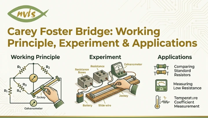
    Carey Foster Bridge: Working Principle, Experiment & Applications

    TL;DR

    • This blog is for engineering students, university freshers, and physics lab learners in India who are studying the Carey Foster bridge experiment and want to actually understand it, not just memorize formulas for exams.
    • A Carey Foster bridge is a precision circuit built to measure very small or nearly equal resistances, something standard Wheatstone bridge struggles to do accurately.
    • The core trick is a slide wire and a clever “swap and re balance” step that cancels out errors from contact resistance and end connections automatically.
    • The balance condition formula looks intimidating at first, but it comes from the same null deflection logic as Wheatstone bridge, just applied twice.
    • This 1872 experiment is still on nearly every Indian engineering physics syllabus in 2026 because it builds measurement intuition that digital instruments hide from you.
    If you have opened your first year engineering physics lab manual and spotted “Carey Foster Bridge Experiment” on the list, you are not alone in feeling a little lost. The name sounds complicated, the circuit diagram looks busy, and the formula involves symbols like l1, l2, P, Q, R, and S that seem to appear out of nowhere. This guide breaks the entire concept down from scratch, starting with what problem this bridge actually solves, before walking through circuit, experiment, and math behind carey foster bridge in plain, step by step language. By the end, you will understand not just how to perform the carey foster bridge experiment for your practical exam, but why it works and where this kind of precision measurement thinking still matters in 2026.

    Also read:

    What Is a Carey Foster Bridge

    Think about trying to compare the weight of two objects that are almost identical, say, two mobile phones from the same model. A regular kitchen scale will not help much here. It might show both as “180 grams” even if one is actually 2 grams heavier. To catch that tiny difference, you would need a much more sensitive balance, one built specifically to detect small differences rather than measure absolute weight. That is exactly the problem Carey Foster bridge solves, except with electrical resistance instead of weight. A Carey Foster bridge is an electrical circuit primarily used to measure low resistances and compare two nearly equal resistances with high precision. It was invented by British physicist George Carey Foster in 1872, as a modification of Wheatstone bridge, which was already a well known tool for resistance measurement at time. Foster introduced the modified bridge in 1872 in his paper On a Modified Form of Wheatstone’s Bridge, and Methods of Measuring Small Resistances. The keyword here is “modified.” Carey Foster bridge did not throw out the Wheatstone bridge concept and start fresh. It took the same null deflection principle and added one important component, a sliding wire, to fix a specific weakness. Understanding that weakness is the fastest way to understand why this bridge exists at all.

    Why Wheatstone Bridge Falls Short

    Before the slide wire trick makes sense, you need to know what a Wheatstone bridge actually does and where it struggles. A Wheatstone bridge works on a simple idea called null deflection. You arrange four resistances in a diamond shape, connect a battery across one diagonal and a galvanometer across another, and adjust one of the resistances until the galvanometer shows exactly zero current. At that exact balance point, a simple ratio relationship holds between four resistances, and you can calculate the unknown one using the other three known values. This works beautifully when you are measuring resistances in medium range, roughly a few ohms to a few thousand ohms, and when values you are comparing are reasonably different from each other. But it runs into trouble in two specific situations that matter a lot in real measurement work. First, when resistance you are measuring is very low, resistance of connecting wires and contacts themselves becomes large enough, relative to what you are measuring, to throw off the result. A wire’s own resistance, which is usually too small to matter, suddenly becomes a significant source of error. Second, when you are comparing two resistances that are almost identical, Wheatstone bridge’s sensitivity is not sharp enough to detect a small gap between them. Near-equal resistances produce only a very small change in the galvanometer reading around the balance point, making the exact null position harder to determine accurately. Carey Foster’s insight was that both problems could be solved with the same fix, a slide wire of uniform resistance placed between two of the bridge’s arms, combined with a simple swap and recheck measurement technique. That is the entire working principle of carey foster bridge in one sentence, and the next section unpacks exactly how it plays out in circuit.

    Carey Foster Bridge Working Principle and Circuit

    Picture Wheatstone bridge’s diamond shape, but with one important change. Instead of four fixed resistors sitting at four corners, Carey Foster bridge places a uniform slide wire, usually one metre long, stretched along a metre scale between two of its arms. A movable contact called a jockey can slide freely along this wire, and it connects to the galvanometer. The circuit has four resistance positions. Two of them, labelled P and Q, are known resistances chosen to be nearly equal to each other, often using a resistance box or two matched coils. The other two positions, X and Y, hold resistances you actually want to compare, one of which is usually a known standard and other unknown resistance you are trying to measure. At both ends of slide wire sit thick copper strips, sometimes called busbars, whose resistance is close enough to zero to be ignored. These copper strips exist purely to connect slide wire cleanly into the rest of the circuit without adding their own resistance into measurement. Here is where the null deflection principle from Wheatstone bridge comes back into play. You pass current through the circuit using a battery and a plug key, then slide jockey along wire until the galvanometer shows zero deflection, meaning no current flows through it. At that exact point, the bridge is balanced, and the same ratio logic that governs a Wheatstone bridge applies here too. But Carey Foster bridge does not stop at one balance reading. It takes a second reading after swapping positions of X and Y, and this second step is where real precision comes from. The next section explains exactly why this swap matters so much.

    Carey Foster Bridge Experiment Step by Step

    If you are heading into the lab for this practical, here is a procedure laid out in order you will actually perform it, along with what is happening physically at each stage. You begin by setting up apparatus: Carey Foster bridge itself with its metre long slide wire, a resistance box, a galvanometer, a battery with a plug key, a thick copper strip, connecting wires, Repeat this process, this time replacing copper strip with your unknown resistance wire to measure that wire’s diameter. Start by connecting known resistances P and Q on either side such that their ratio is close to one, meaning P and Q should be nearly equal. This keeps the bridge sensitive across the full length of slide wire rather than bunching all sensitivity near one end. The experiment is normally performed in two stages. First, a known standard resistance is used to determine the resistance per unit length (σ) of the slide wire. After this calibration, the known standard is replaced with the unknown resistance, and the balancing procedure is repeated to determine its value. Now comes the defining move of this experiment. Swap positions of copper strip and known resistance, so whichever gap had copper strip now has resistance, and vice versa. Slide jockey again to find a new null point, and note this position as l2. distance between l1 and l2 corresponds directly to resistance per unit length of slide wire, once you know the value of resistance you used. Repeat this process, this time replacing copper strip with your unknown resistance wire in place of known resistance box value, to find unknown resistance itself using the same swap and balance method. Finally, measure length and diameter of unknown wire using a metre scale and screw gauge, since these values feed into calculating specific resistance, also called resistivity, of wire’s material.

    Understanding End Correction

    This is part of the Carey foster bridge experiment that trips up most students, not because the concept is hard, but because textbooks usually explain it using only symbols. Here it is in plain language first. When you connect a resistance into one of the gaps of a bridge, that connection is not perfectly resistance free. metal strips, screws, and contact points at each end of slide wire add a tiny bit of extra, unwanted resistance that gets mixed into your reading. This unwanted extra resistance is called end resistance or end correction, and if left unaccounted for, it quietly throws off your final answer. Here is an elegant part of Carey Foster’s design. That end resistance error exists whether you measure copper strip position or resistance box position, and crucially, it exists in the same way both times. So when you take a second reading after swapping X and Y, the end correction error appears identically in both readings. When you then look at the difference between l2 and l1 rather than either value on its own, that shared error cancels itself out completely. You never need to measure or calculate end resistance separately. The swap and subtract method handles it automatically, which is precisely why Carey Foster bridge is so much better at low resistance and near equal resistance measurements than a plain Wheatstone bridge. This is genuinely one of more beautiful pieces of measurement design in classical electrical experiments. Instead of trying to eliminate an error directly, Foster designed a procedure where error cancels itself through subtraction.

    Balance Condition and Formula Derivation

    Now that swap logic makes intuitive sense, the formula itself becomes much easier to follow. It comes directly from applying Wheatstone bridge balance condition twice and comparing two results. In a standard Wheatstone bridge, the balance condition is P/Q = R/S, meaning the ratio of one pair of arms equals the ratio of the other pair at the null point. In Carey Foster bridge, “R” and “S” arms are effectively X plus a length of slide wire, and Y plus remaining length of slide wire. If sigma (σ) represents resistance per unit length of slide wire, and l1 is the first balance point measured from the left end, the balance condition for first reading works out to a relationship between P, Q, X, Y, l1, and σ. When you swap X and Y and take a second reading at l2, you get a second equation with the same structure, just with X and Y exchanged and l1 replaced by l2. Because P and Q, and underlying physical setup, stay exactly the same between both readings, two equations share the same left hand side. That means their right hand sides must be equal too. When you set them equal and simplify algebraically, most of terms cancel out, leaving a strikingly simple final relationship: X minus Y equals σ multiplied by (l2 minus l1) In words, the difference between two resistances X and Y is simply equal to the resistance of the length of slide wire lying between two balance points. This is a balance condition formula that every carey foster bridge experiment lab manual will ask you to derive and apply. Once you know σ, resistance per unit length of wire, you can find any unknown resistance by measuring balancing lengths before and after swapping. And once you know unknown wire’s resistance, its specific resistance, or resistivity, can be calculated using standard formula R equals rho L divided by pi r squared, where L is wire’s length and r is its radius from screw gauge measurement.

    Carey Foster Bridge vs Wheatstone Bridge vs Kelvin Bridge

    Since exam questions and viva sessions often ask students to distinguish between these three, here is a clear side by side comparison.
    Feature Wheatstone Bridge Carey Foster Bridge Kelvin Double Bridge
    Best suited for Moderate resistance measurements Low resistances and near equal resistance comparison Very low resistances (typically below 1 ohm)
    Key structural feature Four fixed resistance arms Slide wire inserted between two arms Second set of ratio arms to cancel lead and contact resistance
    Handles contact/end resistance error No, this limits its precision at low values Yes, cancelled automatically via swap method Yes, cancelled through double ratio arm design
    Typical use case General lab resistance measurement, strain gauge circuits Comparing nearly identical resistances, finding specific resistance of wires Measuring resistance of cables, contacts, and connectors
    Three bridges are best understood as a family, not rivals. Carey Foster bridge is essentially a specialized, higher precision form of Wheatstone bridge, while Kelvin Double Bridge takes concept further still, specifically engineered to eliminate effect of contact and lead resistances when measuring very low resistances. Each one exists because the previous design had a specific blind spot that engineers needed to close.

    Advantages, Limitations, and Precautions

    Like any measurement tool, Carey Foster bridge has strengths worth appreciating and limitations worth knowing before your practical exam or viva. On the advantage side, this bridge delivers genuinely high precision for the specific job it is designed for. Because measurements are based on locating a null point rather than estimating a scale reading, observational errors are reduced. swap and subtract method eliminates end correction and contact resistance errors without any extra calculation. The apparatus itself is also low cost and low maintenance, since it uses simple components like a slide wire, a galvanometer, and a resistance box, all of which are widely available in college labs across India. On the limitation side, slide wire needs periodic calibration, since repeated sliding of jockey contact can wear down wire’s surface over time and change its resistance per unit length slightly. The bridge is also sensitive to temperature, since resistance of both slide wire and wire being tested can shift if the room heats up during a long measurement session. It is a manual, DC only method, meaning it is not suited for AC resistance or impedance measurements, and it takes noticeably longer to perform than simply plugging a wire into a digital multimeter. A few precautions make a real difference to your results. Keep the balance point confined to the middle third of slide wire whenever possible, since sensitivity is highest there and lowest near ends. Never let jockey drag along wire, press it down briefly at each test point instead, since dragging scratches wire and changes its resistance over time. Always include a plug key in the battery circuit and only close it briefly while taking readings, since prolonged current flow heats wire and drifts your balance point. Keep P and Q resistances genuinely close in value, since a large mismatch between them reduces bridge’s overall sensitivity.

    Real World Applications in 2026

    It is fair to ask why a 150 year old measurement technique still matters when digital micro ohmmeters and four wire Kelvin measurement systems can give you a resistance reading almost instantly. The honest answer has two parts, one practical and one educational. On the practical side, underlying null deflection and swap cancellation principles behind Carey Foster bridge are still embedded in how precision resistance and strain measurement instruments are designed today, even when the interface is now a digital display instead of a galvanometer needle. Modern four-wire Kelvin sensing addresses the same measurement challenge reducing errors caused by lead and contact resistance but does so using a different electrical approach. this using separate current and voltage paths, the Carey Foster Bridge reaches a similar goal through its swap-and-balance method to cancel out contact and lead resistance errors, exactly what Foster’s swap method achieved with a slide wire in 1872. The bridge circuit family this experiment belongs to also continues to matter directly in fields like strain gauge measurement, where sensors used in load cells, pressure sensors, and structural health monitoring systems still rely on bridge configurations to detect tiny resistance changes with high sensitivity. On educational side, and this is part most students underestimate, carey foster bridge experiment remains on nearly every Indian engineering physics syllabus, from AKTU to BIT Mesra to Delhi University affiliated colleges, precisely because it forces you to understand where measurement error comes from and how deliberate procedure design eliminates it. A digital multimeter hides all of this from you. You press a button and get a number, with no insight into contact resistance, end correction, or sensitivity trade offs. This experiment builds an intuition for precision measurement that becomes genuinely valuable the moment you step into any lab, quality control floor, or calibration facility in your career. Several Indian institutes now provide access to Virtual Labs simulations that allow students to practice the Carey Foster Bridge experiment before or alongside physical laboratory sessions., allowing students to perform simulated Carey Foster Bridge experiments online before or alongside physical laboratory sessions, now also offer simulated versions of this experiment online, letting students practice balancing and swapping procedure digitally before or alongside physical lab sessions, a genuinely useful 2026 era addition to how this century old experiment is taught.

    Why This Experiment Still Matters: Career Pathways for Indian Engineering Students

    If you are doing this experiment as part of your first year B.Tech or B.E. physics lab, it is worth connecting it to where this kind of thinking leads professionally, because precision measurement is a real, well paying career track in India, not just a lab exercise you forget after the exam. Students who genuinely enjoy logic behind bridge circuits, error cancellation, and precision measurement often find a natural fit in instrumentation and control engineering, a specialization offered as a dedicated B.Tech branch or as electronics and instrumentation engineering at institutes across the country. This field centers on science and technology of measurement and control, spanning sensors, transducers, control systems, automation, electronics, and signal processing, all of which trace their conceptual roots back to exactly the kind of null deflection Carey Foster bridge teaches. career outcomes are genuinely solid for students entering this space. In 2026, instrumentation graduates increasingly work as specialists who design and manage sensor networks and control systems powering automated factories, smart cities, and sustainable energy plants, roles that barely existed in this form a decade ago. Entry-level instrumentation engineers can find opportunities across manufacturing, energy, automation, and process industries, with salaries varying widely by employer, location, and qualifications that vary by employer, location, and qualifications, with experienced professionals earning substantially more as they move into specialized roles. Government and public sector opportunities are also significant in this space. Public sector undertakings including ONGC, BHEL, and SAIL regularly hire instrumentation engineers, typically through GATE qualified recruitment, making this one of more stable long term career routes available to engineering graduates who build a strong foundation in measurement principles early on. Beyond core instrumentation roles, this foundational understanding of precision measurement also feeds naturally into calibration laboratories, quality control departments in manufacturing, semiconductor testing facilities, and research roles in national physical science institutions, all of which value engineers who understand measurement error at a conceptual level rather than only knowing how to read a digital display.

    Conclusion

    The Carey Foster bridge experiment can feel like just another entry on a long physics practical list, but thinking behind it is genuinely elegant once broken down step by step. It takes familiar null deflection logic of Wheatstone bridge and adds a slide wire and a simple swap procedure that automatically cancels out end correction and contact resistance errors, letting it measure low and near equal resistances with a precision original Wheatstone design could never achieve on its own. Understanding why each step of procedure exists, rather than memorizing formula X minus Y equals sigma times l2 minus l1 in isolation, is what will actually help you in your viva, your practical exam, and any future work involving precision instrumentation. This 1872 invention still earns its place on Indian engineering syllabi in 2026 because the core idea behind it, cancelling systematic error through careful procedural design rather than expensive equipment, remains exactly how modern precision measurement instruments are engineered today. Next time you are in the lab sliding that jockey contact along wire, you are practicing a measurement philosophy that genuinely carries through into real instrumentation and metrology careers.

    FAQs

    Carey Foster bridge is primarily used to measure very low resistances and to compare two nearly equal resistances with high precision, a task where a standard Wheatstone bridge is not accurate enough due to end correction and contact resistance errors.

    Interchanging or swapping positions of two resistances being compared causes unwanted end resistance error to appear identically in both balance readings. When you subtract two readings to find difference, this shared error cancels out automatically, which is the central working principle of carey foster bridge.

    The balance condition formula is X minus Y = σ(l2 minus l1), where X and Y are two resistances being compared, σ is resistance per unit length of slide wire, and l1 and l2 are balance point positions before and after swapping X and Y.

    Wheatstone bridge uses four fixed resistance arms and works well for general medium resistance measurement, while Carey Foster bridge adds a slide wire between two arms and uses a swap and balance procedure specifically to achieve higher precision for low resistances and near equal comparisons.

    Even though digital resistance meters exist, this experiment builds a hands-on understanding of measurement error, end correction, and precision procedure design that digital instruments hide behind a simple numeric display, making it valuable groundwork for instrumentation, metrology, and quality engineering careers.

    Keep balance point in middle portion of slide wire for best sensitivity, avoid dragging jockey along wire to prevent scratching it, keep plug key closed only briefly while taking readings to avoid heating effects, and ensure P and Q resistances used are genuinely close in value.

    Tags: carey foster bridge experiment

    Request a Callback

    Please enable JavaScript in your browser to complete this form.

    No spam. Just a quick call.

    =