






• Nvis Technology
  • Nvis Technology
  • Nvis Technology
  • Nvis Technology
  • Nvis Technology
  • Nvis Technology
Nvis Technology

Head Office

141-A, Electronic complex, Pardesipura,Indore - 452010 India

Phone: +91 73899 00887 , +91 98932 70303

Email:info@nvistech.com

Request a Quote

Looking for a quality and affordable builder for your next project?


    Nvis Technology

    Toll Free

    +91 73899 00887

    We are happy to meet you during our working hours. Please make an appointment.

    • Monday-Saturday: 9:00 AM - 5:30 PM (IST)
    • Sunday: Closed

    Swinburne Test of DC Machine and Its Procedures

    TL;DR

    1. This blog is for electrical engineering students, freshers, and GATE, SSC JE, and RRB JE aspirants who want a clear, practical understanding of the Swinburne test of DC machines and how it is performed in a lab.
    2. Swinburne test is an indirect, no load method used to find efficiency of a DC shunt or compound machine without physically loading it, which saves power and protects large machines from damage during testing.
    3. The core idea is simple: run a machine as an unloaded motor, measure the small amount of power it still draws, treat that as constant loss, and then use this one number to predict efficiency at any load, even full load, without ever applying that load.
    4. The test has real limitations. It ignores rise in iron loss at full load and cannot confirm safe commutation or temperature rise under actual working conditions, so engineers pair it with judgment, not blind trust.
    5. Understanding this test builds foundation for machine testing topics that show up repeatedly in GATE Electrical Engineering, SSC JE, and RRB JE exams, and in real testing lab roles at Indian power sector companies.

    Swinburne’s test is a no load, indirect method used to determine efficiency of a DC shunt or compound machine at any load condition, including full load, without actually connecting that load. Named after Sir James Swinburne, the test is one of earliest and most widely taught techniques in Indian electrical engineering laboratories, and it remains a fixture in both classroom experiments and competitive exam syllabi. This blog explains what Swinburne test of DC machines involves, walks through its circuit and procedure step by step, works through a complete numerical example, and covers where this topic fits into GATE, SSC JE, and RRB JE preparation along with career relevance in India’s power sector.

    Also Read,

    What Is the Swinburne Test of DC Machine, Really?

    Picture a large DC motor at a power plant, something rated at 500 kW. To directly measure its efficiency, you would need to connect a full mechanical load capable of absorbing that much power, plus instruments to measure input and output separately. That kind of setup is expensive, time consuming, and honestly a bit risky for a routine test.

    Swinburne figured out a shortcut. Instead of loading the machine fully, run it as a motor with no load at all. At no load, the machine still draws a small amount of current from supply, just enough to overcome its own internal friction, windage, and core losses. Since there is no mechanical output being delivered, every bit of that input power is going into losses.

    Here is the clever part. Most of these losses, like iron loss, friction, and windage, stay roughly constant whether the machine is lightly loaded or fully loaded, as long as speed and flux stay the same. So if you measure these losses once at no load, you can add them to load dependent copper losses at any current level and calculate efficiency at that load, all without ever connecting a real load. That is the entire logic behind the Swinburne test of a dc machine, and it is why the test is also called a no load test.

    This approach works specifically for DC shunt and level compound machines because their field flux stays practically constant regardless of load. A takeaway worth remembering: Swinburne’s test does not measure efficiency directly, it predicts it using losses measured under a much simpler condition.

    Circuit Diagram and Working Principle

    The test circuit is refreshingly simple compared to what it achieves. A DC shunt machine is connected across a DC supply and runs as an unloaded motor. Two ammeters are placed in circuit, one in main supply line to record total no load current drawn from supply, and one in shunt field circuit to record field current separately. A voltmeter reads supply voltage, and a rheostat in field circuit lets you fine tune speed to machine’s rated value.

    Once connections are made and the motor is running at rated voltage and rated speed with no load on its shaft, three quantities are recorded: supply voltage V, total no load line current I0, and shunt field current Ish. Since field winding and armature are in parallel across supply, current actually flowing through armature at no load is different between two readings.

    No load armature current, Ia0 = I0 minus Ish

    This small no load armature current still causes a copper loss in armature winding, calculated as Ia0 squared multiplied by armature resistance Ra. Everything else the machine draws at no load, that is, input power minus shunt field loss minus this armature copper loss, gets grouped together as constant loss.This constant loss includes iron loss, friction loss, windage loss, and shunt field copper loss. In a shunt machine, the field copper loss remains approximately constant because the field current is nearly constant.

    Constant loss, Pc = V I0 minus (I0 minus Ish) squared multiplied by Ra

    Once a PC is known, you have everything you need. For any load current I want to analyze, new armature current becomes I minus Ish for motoring operation, new armature copper loss is calculated from that current, and adding it to Pc gives total losses at that load. Efficiency then follows from basic input minus losses over input relationship.

    Beginner takeaway: think of Pc as a fixed overhead cost machine pays just to keep spinning, and copper loss as a variable cost that grows with load. Once you know fixed cost, predicting total cost at any load becomes simple arithmetic.

    Step by Step Procedure for Swinburne’s Test

    Running actual experiments follows a fairly disciplined sequence, and Indian engineering labs typically structure it like this.

    DC shunt machine is first connected as per circuit diagram, with ammeters, voltmeter, and field rheostat correctly placed. Before switching on the supply, the field rheostat is kept at minimum resistance to establish maximum field current and adequate flux. The motor is then started using a suitable starter, which limits the high armature current at starting.

    Power is then switched on gradually using a starter, since a DC shunt motor connected directly across full voltage at standstill would draw a dangerously high inrush current. As the motor picks up speed, rheostat is adjusted until the machine reaches its rated speed at rated supply voltage. This step matters because losses being measured are only valid at conditions the machine is designed to run at.

    Once speed stabilizes, readings of supply voltage V, no load line current I0, and shunt field current Ish are noted down from meters. It helps to take these readings two or three times and average them, since small fluctuations in a live circuit are normal.

    Separately, armature resistance Ra is measured using a low voltage DC supply and voltmeter ammeter method, with machine stationary. Since this test cares about performance under working conditions, measured resistance is often corrected to account for temperature rise expected during actual operation, since copper resistance increases with heat.

    With V, I0, Ish, and Ra all recorded, the machine is switched off safely, and the calculation phase begins using formulas covered in the earlier section.

    Worked Numerical Example

    Numbers make this concept click faster than formulas alone, so here is a complete example using values typical of a mid-sized DC shunt motor used in Indian engineering labs.

    Consider a 220 V DC shunt motor with a no load line current I0 of 5 A, a shunt field current Ish of 1 A, and an armature resistance Ra of 0.5 ohm.

    First, find no load armature current. Ia0 = I0 minus Ish = 5 minus 1 = 4 A

    Next, calculate armature copper loss at no load. Armature copper loss = Ia0 squared multiplied by Ra = 4 squared multiplied by 0.5 = 8 watts

    Now calculate no load input power. Input power = V multiplied by I0 = 220 multiplied by 5 = 1100 watts

    Constant loss is calculated by subtracting the no-load armature copper loss from the total no-load input power. Pc = 1100 − 8 = 1092 W. This value includes the shunt field copper loss along with iron, friction, and windage losses.

    This constant loss of 1092 watts is now assumed to hold at any load. Suppose you want to predict a motor’s efficiency when it draws a full load line current of 20 A from supply.

    New armature current at this load: Ia = 20 minus 1 = 19 A New armature copper loss: 19 squared multiplied by 0.5 = 180.5 watts Total losses at full load: Pc plus new armature copper loss = 1092 plus 180.5 = 1272.5 watts Total input at full load: 220 multiplied by 20 = 4400 watts Output power: Input minus total losses = 4400 minus 1272.5 = 3127.5 watts

    Efficiency = Output divided by Input = 3127.5 divided by 4400 = approximately 0.7108, or 71.08 percent

    Notice what just happened. Every single reading in this calculation came from a no load test, yet you now have a full load efficiency figure without ever physically loading the motor to 20 A. That is the practical payoff of the swinburne test.

    Advantages and Limitations of Swinburne’s Test

    Every testing method involves trade offs, and Swinburne’s test is no exception. Being upfront about both sides helps you use test correctly rather than treating it as a universal solution.

    AspectAdvantageLimitation
    Power requirementVery low, since machine runs unloadedCannot verify behavior at high current draw
    Time and setupQuick, minimal equipment, ideal for large machinesRequires a separate resistance measurement step
    Efficiency predictionEfficiency at any load can be predicted from one testAssumes constant losses do not change with load, which is only approximately true
    Iron loss accuracySimple to calculate at no loadArmature reaction increases iron loss at full load, an effect this test ignores
    Commutation and heatingNot applicable hereCannot confirm safe commutation or actual temperature rise under real load
    Machine typeWorks well for shunt and level compound machinesNot usable for series machines, since they cannot run safely at no load

    On the advantage side, the biggest win is the economy. Testing a large machine under full mechanical load, sometimes hundreds of kilowatts, would demand load banks, cooling arrangements, and significant electricity consumption. Swinburne’s test sidesteps all of that by drawing only a fraction of rated power from supply.

    On the limitation side, assumption of constant losses is the test’s biggest weak point. In reality, the armature reaction distorts flux distribution at full load, which pushes iron loss somewhat higher than what was measured at no load, sometimes by a noticeable margin. The test also offers zero insight into commutation quality or winding temperature rise under sustained full load, both of which matter enormously for a machine’s real world reliability. This is exactly why Swinburne’s test is not the final word on a machine’s performance, but rather a fast, economical first estimate.

    Takeaway worth remembering: use Swinburne’s test for quick efficiency prediction and preliminary loss separation, but pair it with a load test or Hopkinson’s test when commutation and thermal behavior genuinely need to be verified.

    Swinburne’s Test vs Hopkinson’s Test vs Brake Test

    Students often confuse Swinburne’s test with other DC machine testing methods taught alongside it. A quick comparison clears this up fast.

    FeatureSwinburne’s TestHopkinson’s TestBrake Test
    Loading methodNo load, indirectTwo machines mechanically coupled, regenerative loadingDirect mechanical loading with a brake
    Power neededVery lowLow, since power is largely recirculated between machinesHigh, full load power actually consumed
    Machines requiredOne machineTwo identical machinesOne machine
    Temperature rise dataNot availableAvailable, since machines run under real load for extended periodsAvailable
    Commutation checkNot possiblePossible under real loadingPossible
    Best suited forQuick efficiency estimate on large shunt or compound machinesDetailed testing of two identical machines togetherSmall machines where direct loading is practical

    Swinburne’s test wins on simplicity and economy. Hopkinson’s test, also called back to back test, addresses temperature and commutation blind spots by actually loading two identical machines against each other, though it needs two machines of same rating, which is not always available. A brake test is the most direct approach but only practical for smaller machines where a mechanical brake can safely absorb power. In an Indian testing lab, all three often appear as separate experiments precisely because each fills a gap others leave open.

    GATE, SSC JE, and RRB JE Exam Relevance

    For students preparing for GATE Electrical Engineering, DC machines carry consistent weightage year after year, and Swinburne test question of dc machine shows up frequently as a numerical problem rather than a purely theoretical one. Typical question patterns ask you to calculate constant loss from given no load readings, then use that to find efficiency at a specified full load current, exactly the kind of calculation walked through in the numerical example above. Getting comfortable with algebra of Ia0 = I0 minus Ish and constant loss formula pays off directly in exam scoring.

    SSC JE and RRB JE electrical papers tend to test this topic at a slightly more conceptual level, often through objective questions on why the test cannot be used for series machines, what constant loss physically represents, or which losses test assumes remain unchanged with load. Since these exams favor concise, accurate recall over multi step derivations, understanding reasoning behind each formula, not just memorizing it, tends to serve candidates better than rote learning.

    Both exam tracks also occasionally test comparison between Swinburne’s test, Hopkinson’s test, and direct loading, so table earlier in this blog doubles as solid revision material. A beginner friendly takeaway here: exam setters love this topic because it rewards genuine understanding over memorization, so working through a few numericals yourself, similar to example above, is more useful than reading formulas passively.

    Career Relevance in India’s Power and Electrical Testing Sector

    Beyond exams, the Swinburne test reflects a habit of thinking that Indian electrical engineers use throughout their careers, which is predicting performance efficiently rather than testing everything in an expensive, time consuming way. Testing and quality roles at PSUs like BHEL, NTPC, and Power Grid Corporation regularly involve exactly this kind of no load and indirect testing on motors and generators before they are commissioned into service.

    Beyond exam preparation, the concepts learned through DC machine testing can also support careers in electrical testing, maintenance, manufacturing, and power engineering. For students, the practical value of the Swinburne test lies more in building an understanding of machine losses, efficiency, and testing methods than in directly qualifying for a particular job Junior Engineer and Assistant Engineer positions filled through SSC JE and RRB JE follow 7th Pay Commission structure, generally starting around 35,400 rupees basic pay at Junior Engineer level, rising to higher pay bands at Assistant Engineer level, with gross monthly salaries commonly falling between 50,000 and 90,000 rupees once allowances are included.

    Private sector opportunities have expanded meaningfully too, particularly in India’s growing renewable energy and EV manufacturing space, where power electronics and motor testing skills, the same fundamentals built through experiments like the Swinburne test, are in strong demand. Engineers with hands-on testing experience and machine fundamentals often find these concepts directly applicable when evaluating motor efficiency for EV drivetrains or industrial automation systems. A solid grip on foundational DC machine testing, in other words, keeps paying dividends well beyond exam hall.

    Conclusion

    Swinburne test of DC machine solves a genuinely practical problem: how do you find a large motor’s efficiency without cost and risk of loading it fully? By running a machine unloaded, measuring its small no load losses, and treating those losses as roughly constant across load conditions, the test lets you predict efficiency at any load, including full load, using just a handful of simple readings. The method is fast, economical, and easy to set up, which explains why it remains a staple experiment in Indian electrical engineering labs and a recurring topic in GATE, SSC JE, and RRB JE exams.

    At the same time, its assumptions have real boundaries. Iron loss does shift under full load due to armature reaction, and the test tells you nothing about commutation quality or temperature rise under sustained operation, which is why it works best as a quick first estimate rather than a complete performance certificate. Understanding both what the test reveals and what it deliberately leaves out is what separates rote memorization from genuine engineering judgment, and that judgment is exactly what shows up in exam numericals and real testing lab work alike. If you are preparing for GATE or a JE exam, work through a few more numericals on your own using different no load readings until calculation feels automatic rather than memorized.

    FAQs

    Swinburne test is used to determine efficiency of a DC shunt or compound machine at any load, including full load, by measuring its losses at no load and using that data to predict performance under loaded conditions without physically applying that load.

    A DC series motor cannot run safely at no load because its speed would rise to dangerously high, potentially damaging levels without a load to hold it in check, and since Swinburne’s test requires a running machine unloaded, it simply cannot be applied to series machines.

    Constant loss in the Swinburne test includes iron losses, friction and windage losses, and shunt field copper loss. These are treated as approximately constant when the machine operates at nearly constant voltage, speed, and flux.

    Armature copper loss is calculated by squaring armature current and multiplying it by armature resistance, written as Ia squared multiplied by Ra, using no load armature current for initial constant loss calculation and load specific armature current for efficiency at any given load.

    The test assumes constant losses remain unchanged from no load to full load, which is not entirely accurate since armature reaction increases iron loss under load, and it also cannot verify safe commutation or actual temperature rise during sustained full load operation.

    Yes, Swinburne’s test appears regularly in GATE Electrical Engineering as numerical problems involving efficiency calculation, and in SSC JE and RRB JE papers as conceptual questions on constant loss and machine applicability, making it a consistently high value topic across these exams.
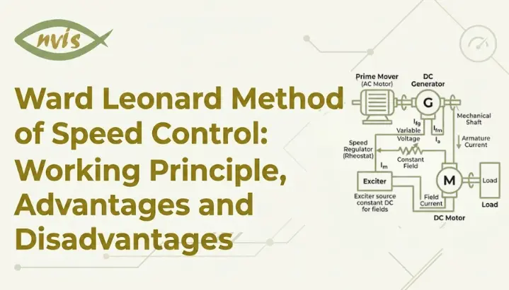
    Ward Leonard Method of Speed Control: Working Principle, Advantages and Disadvantages

    TL;DR

    1. This blog is for electrical engineering students, GATE and SSC JE aspirants, and freshers who want to understand Ward Leonard method of speed control with a clear, exam ready explanation rather than a dry textbook definition.
    2. Ward Leonard system controls a DC motor’s speed by changing voltage fed to it, using a separate motor generator set instead of resistors or switches.
    3. It became one of the smoothest and widest-range speed-control methods for DC motors and was widely used for decades in elevators, steel mills, mine hoists, cranes, and other demanding industrial applications.
    4. A worked numerical example, comparison table, and India specific industrial context are included to help you connect theory to real plants and real exam questions.
    5. Modern power-electronic drives, including thyristor DC drives and, where AC motors are used, VFDs, have largely replaced Ward Leonard systems.

    Imagine trying to slow down a car by dragging your foot on the road instead of easing off the accelerator. It would work, technically, but you would waste a lot of energy as heat and wear out your shoe fast. Early speed control methods for DC motors had a similar problem. Engineers controlled speed by inserting resistors into the circuit, which wasted power as heat, gave a limited speed range, and could not push the motor above its normal speed smoothly.

    Ward Leonard method of speed control solved this problem by changing strategy entirely. Instead of wasting energy through resistors, it changes voltage supplied to the motor directly, using a dedicated generator built just for that purpose. This single idea, controlling speed through variable voltage rather than variable resistance, became one of most important developments in the history of electric drives.

    This blog breaks down Leonard’s system of speed control the way a mentor would explain it on a whiteboard: starting from everyday logic, moving into technical working, and ending with exact things you need for your GATE, SSC JE, or RRB JE preparation.

    Also Read,

    What Is the Ward Leonard Method of Speed Control?

    Picture two water tanks connected by a pipe. If you want more water to flow through the pipe, you do not squeeze the pipe narrower and force water through it. You simply raise the water level in the first tank, and flow increases naturally with more pressure. Ward Leonard method applies exactly this logic to electricity.

    In a DC motor, speed depends almost directly on voltage applied to its armature. Higher voltage means higher speed, and lower voltage means lower speed, as long as field current stays constant. So instead of restricting current with resistors, Ward Leonard method varies voltage itself, smoothly and continuously, using a generator whose output can be adjusted at will.

    The Ward Leonard method of speed control was introduced by American engineer Harry Ward Leonard in 1891. His idea was simple but powerful. Take a constant speed AC or DC motor, couple it mechanically to a separately excited DC generator, and let that generator supply variable DC voltage to the motor you actually want to control. Change generator’s field current, and its output voltage changes. Change output voltage, and the controlled motor’s speed changes right along with it.

    This is why the Ward Leonard control system is often called an armature voltage control method. The field of the controlled motor remains untouched. For speeds up to the base speed, the Ward Leonard system controls the motor through variable armature voltage while keeping the motor field approximately constant. For speeds above the base speed, motor field weakening can be combined with armature voltage control to achieve a wider speed range.

    Three Machines Behind Ward Leonard System

    To really understand how this system works, it helps to think of it as a small team of three machines, each with one job.

    A driving motor is a constant speed machine that keeps everything running. It is usually a three phase induction motor or a synchronous motor, connected directly to the main AC supply, and it always spins at a fixed speed. Its only job is to provide mechanical power to turn the generator.

    The generator is coupled mechanically to the driving motor, so it always spins at that same constant speed too. But its electrical output is not fixed. By adjusting the generator’s own field current through a small rheostat, its output voltage can be raised or lowered smoothly from zero to its rated value, and even reversed in polarity.

    A controlled motor, sometimes labelled M1 in textbook diagrams, is an actual DC motor whose speed you want to control. It receives its armature supply directly from the generator, while its field winding is separately excited and kept constant. Since motor speed depends on armature voltage, and generator’s voltage is fully adjustable, the controlled motor’s speed becomes fully adjustable too.

    The combination of the driving motor and generator is called the motor-generator (MG) set. Together with the controlled DC motor, it forms the basic Ward Leonard system.

    How Speed Control Actually Happens

    Here is where the system becomes genuinely elegant. A field regulator, a small rheostat connected to the generator’s field winding, is the only control operator needs to touch.

    When the generator’s field current is zero, its output voltage is zero, and the controlled motor stays still. As the operator gradually increases field current using rheostat, the generator’s output voltage rises smoothly from zero. This voltage is applied directly to the controlled motor’s armature, so the motor starts rotating and speeds up in proportion to rising voltage.

    Because the generator voltage can be increased gradually from zero, the motor can start smoothly while its armature current remains within the required limit. Therefore, a separate conventional starting resistor is not normally required in the Ward Leonard arrangement.

    Reversing direction is just as elegant. By reversing the generator’s field current using a simple reversing switch, the polarity of the generator’s output voltage flips. This reverses current through the controlled motor’s armature, which reverses its direction of rotation, all while the motor generator set keeps spinning in the same direction throughout.

    There is one more capability that made this system genuinely ahead of its time. During regenerative braking, the generator output voltage is reduced below the motor’s induced back EMF. The motor then operates as a generator and sends electrical power back through the Ward Leonard set. The generator operates in the opposite energy-conversion direction, ultimately allowing the prime mover to return energy to the AC supply. The Ward Leonard system has inherent regenerative braking capability, although the control arrangement must be designed to provide the required operating conditions.

    Worked Numerical Example

    Numbers make this concept concrete, and this is exactly the kind of question that shows up in GATE and SSC JE papers.

    Suppose a separately excited DC generator in a Ward Leonard system is driven at a constant speed and generates 220 V when its field current is at rated value. This voltage is applied directly to armature of a separately excited DC motor whose armature resistance is 0.5 ohm and whose back EMF constant relates speed and flux such that at 220 V armature voltage and rated flux, motor runs at 1000 RPM while drawing a full load armature current of 20 A.

    If the generator’s field current is reduced so that its output voltage drops to 110 V, and motor’s field flux is kept unchanged, new operating speed can be estimated using the relationship that speed is proportional to armature voltage minus armature resistance drop, divided by flux.

    At 220 V: back EMF equals 220 minus (20 times 0.5), which is 220 minus 10, giving 210 V, corresponding to 1000 RPM.

    At 110 V, assuming the motor continues to drive a constant-torque load, the armature current remains approximately 20 A for simplicity. Therefore, back
    EMF = 110 − (20 × 0.5) = 100 V.

    Since speed is proportional to back EMF when flux is constant, new speed works out to 1000 multiplied by (100 divided by 210), which is approximately 476 RPM.

    This shows core exam skill directly: halving generator’s output voltage very nearly halves motor’s speed, since armature resistance drop is small compared to applied voltage. This proportional relationship between generator field current, generator voltage, and motor speed is exactly what most GATE and SSC JE numericals on Ward Leonard method are testing.

    Ward Leonard Ilgner System

    Large industrial loads rarely stay constant. A steel rolling mill or a mine hoist can demand a sudden, massive surge of power for a few seconds and then fall quiet again. Feeding these spikes directly from the AC supply would cause the whole plant’s voltage to sag and flicker, disturbing every other machine connected to the same supply.

    Ward Leonard Ilgner system solves this by adding a flywheel and a slip ring induction motor to standard setup. During normal, light load periods, induction motor spins flywheel up to speed, storing rotational energy in it. The moment a sudden heavy load hits a controlled motor, that stored rotational energy gets released, so the flywheel momentarily slows down while it takes on part of the load itself, easing the burden on incoming supply. Once demand eases off again, the induction motor quietly spins the flywheel back up, ready for the next surge.

    This arrangement reduces the peak power drawn from the AC supply by allowing the flywheel to supply part of the sudden overload. As a result, the required power rating of the supply-side equipment and driving motor can be reduced compared with a system designed to handle the entire peak load directly. This is precisely why the Ilgner variant found its home in heaviest industrial applications, including blooming mill drives and colliery winders, where individual drive units can run into megawatt range.

    Advantages of Ward Leonard System

    The reason this system dominated precision drives for nearly a century comes down to a genuinely strong list of benefits.

    With appropriate armature-voltage control and motor field weakening, the Ward Leonard system can provide a wide speed range; traditional references commonly quote a maximum-to-minimum speed ratio of about 20:1 to 40:1, depending on the design and control arrangement.

    Starting is gentle by nature, since the generator’s output voltage rises from zero, which means the controlled motor accelerates smoothly and no separate starter is required at all.

    Speed regulation under load is excellent, meaning the motor holds its set speed closely even as mechanical load on it changes.

    Regenerative braking is an inherent capability of the Ward Leonard system. When the motor is driven above the speed corresponding to the applied armature voltage, it can operate as a generator and return electrical energy through the drive system to the supply, provided the control arrangement supports regenerative operation.

    Because of all this, the system was, and in some legacy installations still is, a natural choice for jobs demanding frequent starting, stopping, and direction reversal, such as elevators, rolling mills, and excavators.

    Disadvantages of Ward Leonard System

    None of these benefits came free, and drawbacks are exactly why modern plants have largely moved away from this method.

    The system needs three full electrical machines instead of one, driving motor, generator, and controlled motor, which makes initial cost very high.

    All that extra machinery also means a much larger physical footprint, heavier installation, a costlier foundation, and significantly more floor space than a compact modern drive would need.

    Overall efficiency suffers because power is converted twice, first from AC to mechanical to DC in the generator, and then from DC to mechanical again in the controlled motor, and this inefficiency gets worse when the system runs under light load.

    Three rotating machines mean more maintenance requirements, more noise during operation, and more potential points of mechanical or electrical failure.

    These downsides are precisely why solid state alternatives eventually took over, a shift covered in detail in the next section.

    Applications of Ward Leonard Method

    Despite its bulk and cost, Ward Leonard system found a home wherever precision mattered more than efficiency or space.

    Elevators relied on this system for decades, since it offered smooth speed control and consistent torque, until thyristor drives became widely available in the 1980s.

    Steel rolling mills used it to drive rollers that shape red hot steel, where even slight speed inconsistency can ruin an entire batch of material.

    Mine hoists and colliery winders depended on it for safely raising and lowering personnel and material through deep shafts, where smooth acceleration and reliable braking are safety critical.

    Paper mills used it to keep multiple stages of the manufacturing process running at precisely synchronised speeds, since a mismatch anywhere along the line damages paper.

    Beyond heavy industry, Ward Leonard-type motor-generator systems were also used in applications requiring precise electromechanical positioning, where extremely smooth, precise motion it offered was exactly what gun directing systems needed.

    Ward Leonard System vs Modern DC and AC Drives

    Comparing the classic Ward Leonard method against drives that eventually replaced it makes trade offs much clearer.

    ParameterWard Leonard SystemModern VFD / Thyristor Drive
    Number of machines neededThree (driving motor, generator, controlled motor)One (motor itself, plus a compact electronic converter)
    Physical size and weightVery large, heavy, needs significant floor spaceCompact, panel mounted, minimal footprint
    Initial costHigh, due to extra rotating machinesLower, though power electronics add their own cost
    EfficiencyReduced by double energy conversion, worse at light loadHigh, since power electronic conversion has fewer losses
    MaintenanceFrequent, due to brushes, bearings, and commutators on three machinesMinimal, mostly solid state with far fewer moving parts
    NoiseNoticeable, from rotating machineryVery low
    Response speedSmooth but mechanically limitedExtremely fast, controlled electronically
    Typical modern useLegacy installations, some heavy industrial retrofitsStandard choice in nearly all new industrial drives

    Is the Ward Leonard Method Still Used in India Today?

    Walk through a modern Indian steel plant today and you will rarely find a classic Ward Leonard motor generator set still running main rolling stands. Modern Indian steel plants increasingly rely on PLC-based automation and modern power-electronic drives, including DC drives and VFDs, for rolling-mill and other variable-speed applications, which deliver same precise, wide range speed control Ward Leonard system once provided, but from a fraction of footprint and with far less maintenance overhead.

    This does not make the Ward Leonard method irrelevant. It remains genuinely important for three reasons. First, some older Indian mills, mine hoists, and elevator installations still run on legacy Ward Leonard equipment, and engineers maintaining these systems need to understand exactly how they work. Second, the Ward Leonard system is an important historical foundation for modern variable-speed drive technology, particularly electronic DC drives. Modern VFDs use a different approach based on power-electronic conversion and frequency control of AC motors. Third, and most practically for students, this topic is a recurring favourite in GATE, SSC JE, and RRB JE electrical engineering papers, which means skipping it is not really an option if you are preparing for these exams.

    Understanding the Ward Leonard system, in other words, is less about maintaining old machines and more about understanding the DNA of every drive system that came after it.

    Career Relevance of Ward Leonard Speed Control

    Electrical drives and motor control are not just exam topics. They translate directly into real, well paying career paths in India, and understanding classical systems like Ward Leonard gives you a genuine head start when you move on to studying VFDs, servo drives, and industrial automation.

    Career Relevance for Electrical Engineers

    Understanding DC drives, motor control, regenerative braking, and industrial automation can help electrical engineering students build a foundation for careers in electrical drives, industrial automation, power electronics, and maintenance engineering.

    Specialising further pays off significantly. Engineers who build expertise in industrial automation, PLCs, SCADA systems, or power electronics can access specialised career opportunities because these skills are widely used in modern industrial and electrical systems. Since the Ward Leonard method is an important milestone in the development of variable-speed electrical drives, a solid grasp of it makes concepts like VFD tuning, regenerative braking in EVs, and closed loop motor control noticeably easier to pick up later.

    For students still deciding where to specialise, drives and automation remain one of more resilient tracks in Indian electrical engineering, since virtually every steel plant, cement plant, paper mill, elevator manufacturer, and EV company needs engineers who genuinely understand how motor speed control works, not just how to operate a VFD panel by trial and error.

    GATE, SSC JE, and RRB JE Exam Relevance

    Leonard method of speed control shows up consistently across Indian electrical engineering competitive exams, and it is worth knowing exactly what form these questions usually take.

    Conceptual questions typically test whether you understand that this is fundamentally an armature voltage control method, applicable to DC shunt and separately excited motors, and that it is not used for series or universal motors. Expect direct statements to verify as true or false, along with questions asking you to identify which machine’s field current is actually being varied to control speed, since students often confuse generator’s field with motor’s field.

    Numerical questions, similar to worked examples earlier in this blog, usually give you a generator voltage, an armature resistance, a load current, and a known speed at one voltage, then ask you to calculate the resulting speed at a different generator voltage. A key relationship to remember is that back EMF is proportional to speed when flux is constant, and back EMF equals applied voltage minus armature current times armature resistance.

    Application based questions test whether you know why this method suits loads requiring frequent starting, stopping, and reversal, and why it offers inherent regenerative braking without any additional circuitry, a point that is very commonly tested precisely because it distinguishes Ward Leonard from simpler resistance based control methods.

    Comparison questions often ask you to contrast Ward Leonard with other DC motor speed control methods, namely armature resistance control and field flux control, focusing on efficiency, cost, and speed range as key differentiators.

    Conclusion

    Ward Leonard method of speed control took a simple, honest idea, that motor speed follows armature voltage, and built an entire mechanical electrical system around delivering that voltage smoothly and reliably. It gave engineers a highly effective wide-range, bidirectional speed-control system for DC motors, decades before modern power electronics could perform similar functions in a much smaller package.

    To summarise key points from this blog: system uses three machines working together, a driving motor, a generator, and a controlled motor, with speed adjusted purely through generator’s field current. It excels at smooth, wide-range, bidirectional control and inherent regenerative braking capability when operated in regenerative mode, but pays for this with high cost, large size, and lower efficiency compared to modern drives. Ilgner variant added a flywheel to handle heavy intermittent industrial loads without disturbing the main power supply. And while VFDs and thyristor drives have replaced it in nearly all new Indian installations, the underlying principle remains foundational to every modern variable speed drive in use today.

    If you are preparing for GATE, SSC JE, or RRB JE, make sure you can explain the working principle in your own words, solve a voltage to speed numerically confidently, and list advantages and disadvantages without hesitation. That combination covers almost everything examiners ask about this topic.

    FAQs

    Leonard method of speed control is used to smoothly control speed of a DC motor, in both directions of rotation, across a very wide range. It was historically used in elevators, steel rolling mills, mine hoists, cranes, and paper mills, wherever precise, sensitive speed control mattered more than cost or size.

    The system was introduced by American electrical engineer Harry Ward Leonard in 1891, and it went on to become one of most influential drive control methods of the twentieth century.

    Rarely for new installations. Most Indian steel plants and industries have shifted to VFDs and thyristor based drives, which offer similar precise control from a much smaller footprint. However, some legacy elevators, mine hoists, and older mill drives still run on Ward Leonard systems, and underlying principle remains foundational to how modern drives work.

    The standard Leonard control system uses a motor generator set alone. Ilgner variant adds a flywheel and typically a slip ring induction motor, allowing the flywheel to absorb sudden heavy load demands and release stored energy back into the system, which smooths out supply current fluctuations in large industrial drives.

    The biggest drawbacks are high initial cost from needing three separate machines, large physical size and floor space requirements, reduced efficiency due to double energy conversion, and higher maintenance needs compared to modern solid state drives.

    No. This is a common exam trap. Leonard system of speed control is designed for DC shunt motors and separately excited DC motors, where field can be held constant while armature voltage is varied. It is not a standard method used for series motors.

    It is a recurring topic in DC machines and electrical drives sections of these exams, tested through conceptual questions, numericals relating voltage to speed, and comparison questions against other speed control methods. Understanding it thoroughly also builds foundation for later topics like VFDs and closed loop motor control.

    Request a Callback

    Please enable JavaScript in your browser to complete this form.

    No spam. Just a quick call.

    =