Arduino for Embedded Systems Learning: Setting Up Your First Lab Project

Posted on 23-09-2026 by Tushar Saluja

TL;DR

This blog is for ECE, EEE, and CSE students, freshers, and exam aspirants who want to understand how an Arduino embedded system works and set up their first hands-on lab project.
Arduino board itself is more accurately described as an embedded development platform.
A proper Arduino embedded system setup needs the right board, Arduino IDE, correct driver installation, and one working baseline project before adding sensors.
A worked numerical example on LED resistor calculation and PWM duty cycle shows how classroom formulas map directly onto real Arduino code.
Building even one solid Arduino project strengthens GATE, SSC JE, and RRB JE embedded systems answers, and gives freshers something concrete to show in interviews at PSUs and private embedded companies.

Every electronics student eventually asks the same question. Is Arduino embedded system technology, or is it something separate that sits next to embedded systems in a textbook? The confusion is understandable because many courses introduce embedded systems through microcontrollers such as the 8051 or PIC, while practical labs may then introduce Arduino without clearly explaining how the two relate.

This blog answers that question directly and then walks through setting up your first Arduino based embedded system lab project from scratch. You will learn what happens inside the board, how to install software correctly, and how to wire and code your first working circuit. Along the way, you will work through calculations useful for GATE and SSC JE-style questions, along with India specific career context that most tutorials skip entirely.

By the end, you will have a working lab setup and a clear mental model of where Arduino fits in the broader embedded systems landscape.

Is Arduino an Embedded System?

Arduino boards are embedded development platforms based on microcontrollers, and they can be used to build embedded systems for specific tasks. Understanding the role of the Arduino board and its microcontroller helps clarify the difference.

An embedded system is a combination of hardware and software designed to perform a specific function. For example, a washing machine contains a controller that manages functions such as wash cycles, drum movement, and alerts. It is designed for a dedicated purpose rather than general-purpose computing.

An Arduino board contains a microcontroller that provides the processor, memory, and input-output capabilities required to control connected hardware. On the classic Arduino Uno, the microcontroller is the ATmega328P. When a program is uploaded to the board and components such as sensors, LEDs, or motors are connected, the Arduino can be used to build an embedded system.

However, an Arduino board is more accurately described as an embedded development platform built around a microcontroller. It provides a ready-made hardware and software environment that simplifies the development of embedded applications, particularly for beginners and students.

Therefore, Arduino is best understood as a development platform used to create and learn embedded systems, rather than as a separate category that competes with embedded systems. It allows users to work with real microcontroller hardware without designing a custom circuit board from the beginning.

Arduino vs Traditional Embedded Systems Development

Once you understand Arduino as an embedded development platform, the next useful question is how it compares to the traditional route of embedded systems learning.

In a conventional bare-metal workflow, you may program an 8051 or PIC directly using C or assembly, configure peripherals through registers, and use a programmer or debugger to load and test the firmware, configure peripherals through registers, and use a programmer or debugger to load and test the firmware. This teaches you exactly what is happening at hardware level, but the learning curve is steep for a first year student.

Arduino removes several of these early barriers. The board already has a USB interface, a voltage regulator, and a pre-loaded bootloader that lets you upload code with one click. Arduino IDE hides much of low level register configuration behind simple functions like pinMode and digitalWrite. You still write in C or C++, so programming logic you learn transfers directly to professional embedded work later.

This is why Arduino can be a useful starting point before moving to platforms such as STM32 or bare-metal AVR programming. You get real embedded hardware experience quickly, then dig deeper into register level control once fundamentals are solid.

Aspect	Arduino Development	Traditional Bare Metal (8051/PIC)
Programming language	C/C++ with simplified functions	C or Assembly with direct register access
Upload method	USB, one click upload	External programmer/burner required
Learning curve	Gentle, beginner friendly	Steep, needs hardware register knowledge
Cost to start	Low, single board around Rs 500 to Rs 900	Board plus separate programmer needed
Best suited for	Beginners, rapid prototyping, hobby and lab projects	Students learning register level architecture, production design
Industry relevance	Prototyping, IoT, hobbyist and academic projects	Automotive, industrial, and safety critical production systems

What You Need for Your First Arduino Embedded System Setup?

Before touching any code, gather physical components. A cluttered or incomplete lab setup is the most common reason first projects fail.

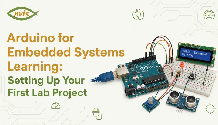
For a basic arduino embedded system setup, you need an Arduino Uno board, which is the most widely supported and documented option for beginners. You also need a USB cable, typically USB Type B on the original Uno, to connect the board to your laptop. A breadboard and a small set of jumper wires let you build circuits without soldering. Finally, keep a few basic components on hand, an LED, a 220 ohm resistor, and a push button, since almost every early tutorial uses these.

Budget wise, a genuine Arduino Uno costs more, but clone boards using the same ATmega328P chip are widely available in India through electronics markets like Lamington Road in Mumbai, SP Road in Bengaluru, or online sellers, usually priced between Rs 400 and Rs 700. For a first lab project, a reputable Arduino-compatible clone can be a cost-effective option, although USB interfaces, component quality, and driver requirements can vary between boards.

Software wise, you only need Arduino IDE, which is free and available for Windows, macOS, and Linux. There is no need for a separate compiler or an external programmer device, which is one of the biggest practical advantages Arduino offers over other microcontroller platforms.

Installing and Configuring Arduino IDE

With hardware in hand, the next step is getting your development environment ready. This is where many beginners get stuck, usually on driver installation rather than software itself.

Download Arduino IDE from the official Arduino website and install it using the standard installer for your operating system. Once installed, connect your Arduino board to your computer using USB cable. Windows will often detect a genuine Arduino automatically, although driver or USB-port issues can still prevent recognition. Clone boards often use a CH340 USB to serial chip instead of the original chip, and Windows sometimes needs a separate CH340 driver installed manually before the board is recognized.

After installation, open Arduino IDE and go to Tools, then Board, and select Arduino Uno from the list. Next, go to Tools, then Port, and select the COM port your board appears under. On Windows this typically looks like COM3 or COM4. On Linux or macOS, it usually appears as something like /dev/ttyUSB0 or /dev/cu.usbmodem.

To confirm everything works, open File, then Examples, then 01.Basics, then Blink. Click the checkmark icon to compile code, then click the arrow icon to upload it. If the onboard LED starts blinking once every second, your Arduino embedded system setup is complete and ready for real projects.

Your First Real Project: LED Control with a Push Button

Blinking built in LED confirms your setup works, but it does not teach interaction. A slightly more meaningful first lab project is controlling an LED using a push button, since it introduces both digital input and digital output in one circuit.

Build circuit by connecting LED’s longer leg through a 220 ohm resistor to digital pin 13, and shorter leg to GND. Connect one leg of the push button to digital pin 2, and the other leg to GND. Using INPUT_PULLUP mode in code avoids the need for an external pull up resistor on button, which simplifies wiring for a first attempt.

const int buttonPin = 2;

const int ledPin = 13;

int buttonState = 0;

void setup() {

pinMode(ledPin, OUTPUT);

pinMode(buttonPin, INPUT_PULLUP);

}

void loop() {

buttonState = digitalRead(buttonPin);

if (buttonState == LOW) {

digitalWrite(ledPin, HIGH);

} else {

digitalWrite(ledPin, LOW);

}

Here is what happens line by line. setup function configures pin 13 as an output for LED and pin 2 as an input with its internal pull up resistor enabled. Inside the loop, digitalRead constantly checks the button’s state. Because of the pull up configuration, the pin normally reads HIGH, and pressing the button pulls it to LOW by connecting it to ground. When code detects LOW, it turns the LED on, and otherwise keeps it off.

This project matters more than it looks. It demonstrates a core embedded systems loop of reading an input, processing a condition, and driving an output, which is exactly the pattern used in far more complex systems, from an elevator controller to an EV battery management system.

Worked Example LED Resistor and PWM Calculation

GATE and SSC JE questions on embedded systems often test whether you can apply basic circuit laws inside a microcontroller context, not just recall definitions. Here is a worked example that combines both.

Problem: An LED with a forward voltage of 2V and a required forward current of 15mA is connected to an Arduino digital pin that outputs 5V. Calculate the required resistor value. Then, if this LED is dimmed using PWM with a duty cycle of 40 percent, calculate its average voltage across the LED.

Step 1: Resistor calculation using Ohm’s Law

The resistor must drop the difference between supply voltage and LED’s forward voltage.

Voltage across resistor = Supply voltage − LED forward voltage

= 5 V − 2 V

= 3 V

Resistance = Voltage across resistor divided by required current Resistance = 3V divided by 0.015A = 200 ohms

Since 200 ohm is not a standard resistor value, the nearest standard value, 220 ohm, is used in practice, which slightly reduces current for safety margin.

Step 2: Average voltage under PWM

PWM does not change peak voltage. Instead, it switches pins on and off rapidly, and PWM controls LED brightness by rapidly switching the Arduino output between 0V and 5V. The duty cycle determines the proportion of time the LED is powered during each cycle. This proportion is called duty cycle.

For a simplified PWM calculation, the average Arduino output voltage is:

Average output voltage = Duty cycle × Supply voltage

= 0.40 × 5 V

= 2 V

This means at 40 percent duty cycle, LED experiences an effective average voltage of 2V, which is why it appears noticeably dimmer than at full brightness, even though actual pin voltage is still switching between 0V and 5V.

This type of numerical combines basic Ohm’s Law with the concept of PWM duty cycle, making it useful practice for electronics and embedded-systems fundamentals.

India Specific Context for Arduino Skills

Arduino experience by itself will not get you a government job, but concepts it teaches map directly onto how embedded systems are tested and used across Indian industry and PSUs.

Organizations such as ISRO, DRDO, BEL, BHEL, and HAL recruit engineers for a range of electronics, electrical, control, embedded, and related technical roles. Arduino projects can provide an early foundation in concepts such as GPIO, sensors, control logic, and microcontroller programming, although production systems use more specialized hardware and development processes. An Arduino project can help students begin developing some of the underlying skills used in these fields. While these organizations use industrial-grade microcontrollers and stricter development processes in production, the underlying logic of reading sensors, applying control conditions, and driving actuators is conceptually similar to what a student learns by wiring an LED and a button to what a student learns by wiring an LED and a button.

On the private-sector side, India’s electric-vehicle industry has created demand for engineers working on embedded systems for areas such as battery management, motor control, and vehicle electronics. Understanding microcontroller-based control systems provides a useful foundation because many EV subsystems rely on embedded control principles. Similarly, India’s Production Linked Incentive scheme for electronics manufacturing has pushed more companies toward in house embedded product design rather than only assembly work, increasing demand for engineers comfortable with hands-on microcontroller development.

For freshers, a portfolio built around genuine Arduino projects, not just tutorials copied without understanding, signals to interviewers that you can move from theory to a working circuit. That single differentiator often matters more in interviews than which specific board or platform you used.

GATE, SSC JE, and RRB JE Exam Relevance

Microcontroller, digital-electronics, and interfacing concepts appear in some technical examination syllabi. Candidates should check the current official syllabus for the specific exam, and Arduino-based learning can reinforce some of the underlying concepts tested in these exams, even though the exams themselves may not mention Arduino by name.

GATE ECE covers relevant digital-system, electronic, and computer-architecture concepts, while the exact treatment of microprocessors, microcontrollers, and interfacing depends on the current syllabus. Learning these concepts through Arduino can make the underlying hardware concepts easier to understand. GATE papers related to electronics and instrumentation cover several concepts that can be reinforced through hands-on microcontroller projects.

For SSC JE Electrical preparation, Arduino can help students strengthen basic electronics and digital concepts through hands-on practice, although the exam syllabus should be followed directly for topic coverage. For RRB JE and other technical recruitment exams, the relevance of microcontroller and embedded concepts depends on the specific discipline and current syllabus rather than platform specific trivia.

The practical advantage of having built even one working Arduino project is that abstract exam topics like ADC resolution, PWM duty cycle, or interrupt handling stop being memorized definitions and become things you have actually observed happening on a breadboard. This noticeably improves both recall speed during exam and confidence during any follow up viva or interview round.

Career and Salary Outlook for Embedded Systems Engineers in India

Embedded systems remains one of more stable and steadily growing career paths for ECE and EEE graduates in India, and starting with Arduino is a legitimate first step toward it.

Freshers entering embedded roles typically start in the range of Rs 4 LPA to Rs 8 LPA at automotive component makers, semiconductor companies, and product engineering firms, with service based companies often on the lower end of that range and specialized product companies on the higher end. Engineers who qualify through GATE and are recruited by organizations such as DRDO for Scientist B positions can start at the Level-10 pay scale, with the basic pay listed at Rs 56,100, alongside strong long term growth and job security. With three to five years of experience, embedded engineers commonly move into the Rs 8 LPA to Rs 15 LPA range, and specialization in automotive embedded systems, particularly around AUTOSAR and CAN protocols for growing the EV and automotive sector, can push packages considerably higher.

The field particularly rewards engineers who combine software skills like C and C++ with genuine hardware understanding, exactly the combination that hands on Arduino based learning builds from the very first lab session. As India’s semiconductor and EV manufacturing base expands under central government incentive schemes, demand for engineers who can comfortably move between code and circuit is likely to keep growing faster than supply of such talent.

Conclusion

Arduino is an embedded development platform built around a microcontroller and can be used to create real embedded systems. Treating it as a practical starting point for embedded learning helps you build fundamentals before moving to more advanced platforms. Setting up your first arduino embedded system lab project, from installing IDE correctly to wiring your first button controlled LED, teaches the basic pattern of reading an input, processing the result, and controlling an output that appears in many embedded systems you will encounter later, from industrial PLCs to EV battery controllers.

Combine that hands-on foundation with exam specific numerical practice and India specific career context covered here, and you have a genuinely well rounded starting point, whether your goal is a GATE rank, a PSU interview, or your first embedded engineering job. Set up your board today, build button LED projects yourself, and treat every future circuit as one more step toward a stronger embedded systems foundation.

FAQs

Is Arduino considered a real embedded system or just a learning tool?

An Arduino-based setup can function as an embedded system when the board, program, and connected hardware are designed to perform a specific task. It is also an excellent learning tool, but these two things are not contradictory, since the board itself contains a real microcontroller doing real embedded work.

Do I need prior programming knowledge before starting arduino embedded system setup?

No prior programming experience is required. Arduino uses a simplified version of C/C++, and most beginners learn programming concepts alongside electronics concepts through guided projects like ones covered in this blog.

Which Arduino board is best for a first embedded systems lab project?

Arduino Uno is a recommended starting board because it has a large amount of tutorials, community support, and compatible components, making troubleshooting far easier for a first time user compared to other boards.

How is Arduino different from microcontrollers used in GATE or SSC JE syllabus topics?

Underlying concepts, such as interfacing, memory, and input output handling, are the same. Arduino simply wraps these concepts in beginner friendly functions, while exam syllabus content often discusses them at a more theoretical or register level, which you can explore further once comfortable with Arduino basics.

Can Arduino projects actually help during placement interviews for embedded roles?

Yes, a well understood Arduino project demonstrates that you can translate theoretical embedded systems knowledge into a working circuit, which can give interviewers evidence that you can apply embedded concepts in practice. The depth of the project and your understanding of the design decisions generally matter more than the specific development board used.

What is the most common mistake beginners make during their first arduino embedded system setup?

Tags: Arduino embedded systems

IoT Microcontroller Projects for Engineering Students: From Sensor to Cloud

Posted on 22-09-202622-09-2026 by Tushar Saluja

TL;DR

This blog is for engineering students, freshers, and GATE/SSC JE aspirants who want to understand what a microcontroller in IoT actually does and how to build a working sensor to cloud project from scratch.
Many smart devices, such as fitness trackers and smart streetlights, rely on microcontrollers to sense, process, and respond to information.
Choosing the right IoT development board depends on your project’s processing, connectivity, power, and peripheral requirements rather than simply following the most popular option.
Building even one complete sensor to cloud project teaches skills directly relevant to GATE, SSC JE, RRB JE, and entry level embedded and IoT roles in India.

Many smart devices, such as fitness trackers and smart streetlights, rely on tiny embedded chips to sense, process, and respond to information. In many iot microcontroller devices, this role is handled by a microcontroller. Understanding how microcontrollers work is therefore useful for engineering students interested in IoT and embedded systems. This blog explains what a microcontroller does for an iot device, how to choose one that’s best suited for your needs and build an entire iot project from sensors through cloud computing. At this stage, you will have an understanding of concepts and a working prototype that you can present and discuss during an interview.

What Is a Microcontroller in IoT ?

A microcontroller used in an IoT device is an integrated circuit that combines a processor core, memory, and peripherals such as GPIO, timers, communication interfaces, and sometimes ADCs on a single chip. It’s designed for performing particular controls and processing functions effectively instead of doing general-purpose computing tasks.

A microcontroller is a component commonly used inside an embedded system and can act as the local controller for an IoT device. It can collect information like temperature, humidity, motion, gas sensor readings; process this information to respond as per programmed parameters. For instance, it may convert an electrical signal from a sensor into a temperature value, activate a fan when the temperature exceeds a set limit, and send the processed data to another device or cloud service using protocols such as MQTT or HTTP.

The microcontroller is ideal for iot because it’s small, cheap and low power consuming. Unlike a typical microprocessor-based system, where memory and peripherals may be provided as separate components, a microcontroller integrates a processor, memory, and many peripherals on a single chip. It reduces total hardware needed for building an iot device.

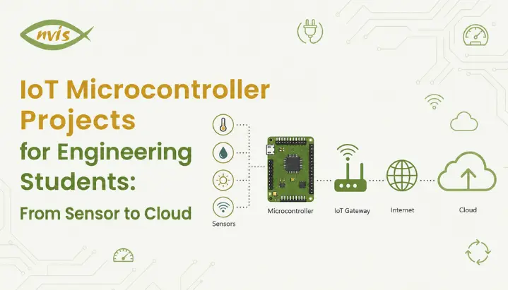
basic role of a microcontroller in an IoT system can therefore be summarized in three stages:

Collect data: Read information from connected sensors.
Process data: Convert and analyze sensor readings according to programmed logic.
Control or communicate: Trigger an action locally or send processed information to another device, gateway, or cloud service.

Thus, microcontrollers provide local intelligence that allows an IoT device to sense its environment, process information, and respond or communicate accordingly.

Why Microcontrollers Matter So Much in IoT Development

This is an interesting question to sit on for a while. Why not just use a regular computer chip for every IoT device. An intelligent drinking water bottle with a reminder function does not require an integrated processor like that found on gaming laptop computers.

This is where the role of a microcontroller in IoT becomes clear. IoT gadgets are usually powered by batteries; they are tiny and need to last for months/years without any repairs. A microprocessor-based system typically requires more supporting hardware and may consume more power than a microcontroller-based design, making microcontrollers a practical choice for many simple, battery-powered IoT devices.

The microcontroller solves it through being designed for that purpose. Many microcontrollers offer low-power sleep modes that can reduce current consumption significantly, while still providing enough processing capability for sensor logic, decision-making, and communication. Low power, low cost and just enough computing is what made IoT development explode the way it did over the past decade.

Scalability is another important factor. Smart city projects may use ten thousand sensors on streetlights, water pipes and traffic lights. Deploying a full computer at every sensing point would often add unnecessary cost, power consumption, and complexity. Microcontrollers are practical for many mass-deployed IoT endpoints where low power, low cost, and local control are important, from college-level projects to industrial monitoring systems.

What Is MQTT in IoT?

MQTT (Message Queuing Telemetry Transport) is an efficient messaging protocol that is commonly used for communication between iot devices, applications, and servers. Publish-subscribe is an example of this communication pattern where a device publishes information on a particular topic that other computers/applications can subscribe for receiving this information.

An MQTT-based IoT application uses an intermediary called a broker to receive messages from publishers and deliver them to subscribers. A sensor node like an iot device (microcontroller) publishes sensor data to a topic like home/livingroom/temperature. MQTT broker receives this message, then forwards it to every client that is subscribed for this particular topic. This allows publishers and subscribers to exchange information without communicating with each other directly.

IoT applications are well suited to use of MQTT as they have low network traffic needs, low bandwidth requirements. It is useful to microcontrollers, battery-powered devices, and systems running on limited or unreliable networks. MQTT also has some small fixed protocol overhead, although the total message size depends on the topic, payload, and other protocol fields.

For instance, an ESP32 based weather station can measure the temperature every ten seconds and publish the reading to home/livingroom/temperature. The MQTT broker receives this information, then sends it on to subscribers like an app and dashboard. Once the dashboard receives the published data, you can view the latest temperature readings online without repeatedly checking the sensor itself.

Thus, MQTT is an effective means to communicate between iot devices/applications by publishing/subscribing/sharing information about sensors via a lightweight topic-based messaging protocol.

How the Sensor-to-Cloud Pipeline Works

Before touching any code, it helps to understand the full journey your data takes in a typical IoT development project. Picture posting a letter. You write it, drop it in a letterbox, it travels through a sorting system, and eventually reaches someone who reads it and reacts. IoT data follows the same logical journey.

Stage 1: Sensing

A sensor is a device that observes something in the physical world and converts it into an electrical signal. Sensors can provide either analog or digital output. For example, an MQ-2 and many soil-moisture sensors can provide analog readings, while the DHT22 communicates digitally with the microcontroller. The microcontroller reads the sensor output and converts or interprets it into useful values.

Stage 2: Processing

This is where microcontrollers in IoT earns its keep. When a sensor provides an analog voltage, the microcontroller can use its ADC, or analog-to-digital converter, to convert that voltage into a digital value that the program can process. Digital sensors such as the DHT22 do not require the same ADC conversion step. It then applies logic. Is the temperature too high? Is the soil too dry? Should an alert be triggered?

Stage 3: Connectivity

Once the microcontroller decides data is ready to be sent, it hands it off to a communication module. This could be a built-in Wi Fi radio, as in ESP32, or an external module connected to a microcontroller that lacks built-in wireless, like a classic Arduino Uno paired with an ESP8266.

Stage 4: Cloud and Visualization

MQTT or HTTP requests carry your data from microcontroller in IoT to cloud platform, where it gets stored, graphed, and made available for users to see on a dashboard or app. This is the part that makes the IoT feel magical, watching a live graph update on your phone because a sensor in your room just took a reading.

Most competitor tutorials stop at “sensor sends data to cloud” without explaining how that handoff actually works. One common way to handle the communication between IoT devices, gateways, applications, and cloud services is MQTT. Other approaches, including HTTP and CoAP, are also widely used depending on the application.

Choosing Right Microcontroller for Your IoT Project

This is where many students get stuck. There are many development boards available, and different tutorials often recommend different options. The choice becomes easier once you know what your project actually requires.

Ask three questions to start with. Is there a built-in wireless capability? Does it have to run for months on a small battery? Does the project require precise timing or real-time control, such as controlling a motor’s speed?

If your requirement is “I need Wi-Fi and want to build a working prototype quickly,” an ESP32 is usually a strong choice for an IoT project. Wi-Fi, Bluetooth support is available, it has a dual core processor, and it is easy to use for beginners with Arduino IDE. This makes the ESP32 a popular choice for college-level IoT development projects.

If your project prioritizes precise timing, real-time control, or advanced peripheral support and you are comfortable using a separate wireless module, an STM32 board can be a suitable choice. STM32 boards, many of which use ARM Cortex-M cores, offer a wide range of peripherals and strong real-time control capabilities. They are commonly used in motor control, industrial automation, and precision measurement applications, which matters for projects involving motor control or precision measurement.

For beginners who want to learn microcontroller programming before moving into wireless projects, the Arduino Uno can be a straightforward starting point.

Microcontroller	Built in Wi Fi/Bluetooth	Best For	Approx. Price (India)	Learning Curve
Arduino Uno	No	Learning basics, sensor interfacing	Rs 450 700	Easiest
ESP32	Yes (Wi Fi + Bluetooth)	IoT projects, cloud connectivity, home automation	Rs 350 600	Easy to Moderate
ESP8266 (NodeMCU)	Yes (Wi Fi only)	Budget IoT projects, simple sensor to cloud setups	Rs 200 350	Easy
STM32 (Blue Pill/F4 series)	No (needs external module)	Motor control, industrial automation, precision projects	Rs 300 1200	Moderate to Advanced
Raspberry Pi Pico W	Yes (Wi Fi)	Python based IoT projects, custom I/O timing	Rs 500 700	Easy to Moderate

A quick clarification many students ask about: is a Raspberry Pi a microcontroller? No, a Raspberry Pi is a microprocessor based single board computer running a full operating system like Linux, while Raspberry Pi Pico is genuinely a microcontroller board. This distinction often shows up in exam questions and interviews, so it is worth remembering clearly.

How to Calculate IoT Battery Life

Numbers help to remember things better so let’s try out some math problems that may appear on an GATE/SSC JE exam and are also relevant for project design.

Suppose you are building a soil moisture monitoring node using an ESP32 that will run on a 2000 mAh battery. Assume the ESP32-based node draws 160 mA during the active five-second period, and this active phase lasts 5 seconds every reading cycle. Between readings, it enters deep sleep mode, drawing only 10 microamps for the remaining 595 seconds of a 10 minute cycle.

Calculate the average current consumption first.
Active phase charge per cycle = 160 mA × (5/3600) h ≈ 0.222 mAh.
Sleep phase charge per cycle 0.01 mA multiplied by equals 0.00165 mAh.
Total charge per 10 minute cycle 0.222 plus 0.00165 equals approximately 0.2237 mAh.
Number of cycles in 24 hours 144 cycles, since there are 144 ten minute intervals in a day.
Total daily consumption 0.2237 x 144 = approximately 32.2 mAh per day.

The theoretical battery life is approximately 62 days, assuming the battery can deliver its full rated capacity and the ESP32 consistently follows the stated current profile. In practice, battery life will be lower because of battery characteristics, voltage regulation losses, Wi-Fi behavior, sensor consumption, and temperature.

This one calculation shows precisely how important deep sleep modes are for actual IoT development. Without sleep mode, the same ESP32 running continuously at 160 mA would drain a 2000 mAh battery in approximately 12.5 hours. That difference, 62 days versus half a day, is the entire reason power management is treated as a core skill in embedded systems and IoT interviews.

How to Build a Sensor-to-Cloud IoT Project

Let’s put everything together into a project structure you can actually build. We will use a temperature and humidity monitoring system, a common and genuinely useful starting project for IoT development.

Components needed: An ESP32 board, a DHT22 temperature and humidity sensor, a breadboard, jumper wires, and a free ThingSpeak or Blynk cloud account.

Step 1: Wire sensor. Connect DHT22’s data pin to a GPIO pin on ESP32, and connect its power and ground pins accordingly. This is the sensing stage of our pipeline.

Step 2: Write reading logic. Using Arduino IDE, write code that reads temperature and humidity values from DHT22 every few seconds. This is the processing stage, where raw sensor data becomes usable numbers.

Step 3: Connect to Wi Fi. Add code that connects ESP32 to your Wi Fi network using your network credentials. Without this step, the microcontroller has no way to reach the outside world.

Step 4: Publish to cloud. Use the platform’s supported API or library to send your readings to a cloud channel or dashboard. Depending on the platform and implementation, the data may be transmitted using HTTP or MQTT.

Step 5: Visualize data. Log in to your ThingSpeak dashboard and watch live graphs update as your sensor sends new readings. If you want to go further, set a threshold, such as an alert if humidity crosses 80 percent, and trigger an email or app notification.

Once you have built this one project end to end, you understand the entire IoT development pipeline well enough to extend it into more advanced ideas, such as a smart irrigation system, an air quality monitor, or an energy consumption tracker for your hostel room.

Microcontrollers in IoT and Industry Relevance in India

For engineering students in India, microcontroller and IoT skills are relevant beyond classroom projects because they are used across embedded, industrial, automotive, and connected-device applications; it’s also relevant for job opportunities and government projects related to the electronics industry.

India’s growth in electronics manufacturing, connected devices, and electric mobility has increased the relevance of hardware, firmware, embedded systems, and connectivity skills. IoT product companies may require engineers with skills in microcontroller programming, sensor interfacing, firmware development, and cloud connectivity.

Organizations such as ISRO, DRDO, BEL, and BHEL work on systems involving embedded electronics, instrumentation, control, monitoring, and related technologies. The specific processors and architectures used vary by project. Although industrial and government systems use hardware and design practices far more sophisticated than a classroom ESP32 project, the basic engineering workflow sensing, processing, communication, testing, and validation remains relevant.

In terms of the private sector, iot development has become one of its specializations among core electronics and computer science jobs done by big companies like automakers that develop connected vehicles and smart factories that use industrial iot for predictive maintenance.

GATE, SSC JE, and RRB JE Exam Relevance

If you are preparing for competitive exams, microcontroller and embedded systems concepts are particularly relevant to GATE Electronics and Communication Engineering and Instrumentation Engineering preparation.

Microprocessor and microcontroller concepts are relevant to GATE preparation, particularly for students studying digital systems, computer organization, and related electronics topics. Check the latest official GATE syllabus for the exact topic coverage, and questions frequently touch on interfacing, memory organization, and input output handling. For GATE Instrumentation Engineering, microprocessor/microcontroller and interfacing-related topics should be studied according to the current official syllabus.

For relevant technical exams such as GATE and RRB JE, students should review fundamentals such as microprocessor and microcontroller concepts, digital electronics, ADC/DAC, and interfacing where these topics are included in the applicable syllabus. Important areas may include basic microcontroller architecture, differences between microprocessors and microcontrollers, ADC/DAC characteristics, and fundamental embedded-system concepts, difference between microprocessors and microcontrollers, ADC and DAC characteristics, and fundamental embedded system concepts. These questions are usually conceptual rather than heavily numerical, which means a strong grasp of definitions and practical understanding, exactly what this blog has built so far, goes a long way.

A practical exam strategy: do not just memorize that a microcontroller has a CPU, RAM, ROM, and I/O on a single chip. Understand why that integration matters, as we covered in earlier sections, because exams increasingly frame questions around application and reasoning rather than pure recall.

Career and Salary Guidance for Aspiring IoT Engineers

Once you have a working IoT development project under your belt, it becomes a genuine asset for placements and interviews, not just a lab submission.

Freshers entering IoT and embedded roles in India can typically expect starting salaries in the range of Rs 3 to 8 LPA, depending on the company, your project portfolio, and your grasp of both hardware and cloud side skills. Roles at larger product companies and multinational corporations tend to sit at the higher end of this range, especially for candidates who can demonstrate hands-on project experience rather than just theoretical knowledge.

As you gain experience, typically in the 4 to 7 year range, with experience, professionals who combine embedded development with cloud integration, IoT protocols, security, or industrial IoT skills may qualify for more advanced roles with higher compensation. Specializing further into edge computing, firmware security, or industrial IoT tends to open even higher paying senior roles later in a career.

For students specifically, practical advice is this: a single well documented sensor to cloud project, complete with a GitHub repository, a short demo video, and a clear explanation of your design choices like power calculation we walked through earlier, often matters more in interviews than a long list of half finished project titles on a resume.

Conclusion

Understanding a microcontroller in IoT is really about understanding one small but powerful idea: a tiny, efficient chip can sense the physical world, make sense of that data, and connect it to the cloud, all while running on a fraction of the power a regular computer would need. We walked through what a microcontroller actually does, why it matters for iot microcontroller at scale, how data travels through sensor to cloud pipeline using protocols like MQTT, and how to choose the right board for your specific project. We also worked through a real battery life calculation and a complete project structure you can build today.

The best next step is not to read another article, it is to order a DHT22 sensor and an ESP32 board, and build the project we outlined above. Once you see your own sensor data update live on a cloud dashboard, IoT development stops being an abstract topic and becomes a skill you genuinely own. Share your first project results or questions in comments, and start building.

FAQs

What is a microcontroller in IoT, in simple terms?

A microcontroller in IoT is a small, self-contained chip that reads data from sensors, processes it, and either acts on it directly or sends it to the cloud through a communication module. It combines a processor, memory, and input output pins on a single chip, making it ideal for compact, battery powered IoT devices.

Which microcontroller is best for beginners starting IoT development?

ESP32 is generally the best starting point because it has built in Wi Fi and Bluetooth, works with beginner friendly Arduino IDE, and is affordable enough for student projects. If you want to first understand microcontroller programming without wireless features, an Arduino Uno is a solid teaching board before moving to ESP32.

Is a Raspberry Pi considered a microcontroller?

No, a standard Raspberry Pi is a microprocessor based single board computer that runs a full operating system like Linux. Raspberry Pi Pico, however, is genuinely a microcontroller board, and this distinction is worth remembering for exams and interviews.

How does MQTT help in IoT microcontroller projects?

MQTT is a lightweight publish subscribe protocol that lets a microcontroller in IoT send data to a specific topic, which any subscribed application or dashboard can instantly receive. It is designed for constrained networks, with relatively low protocol overhead and support for lightweight messaging, which makes it ideal for battery operated IoT devices.

Are microcontroller and IoT topics important for GATE and SSC JE exams?

Yes, Microcontroller and embedded-system concepts are relevant to some GATE and technical-exam syllabi, but the exact coverage varies by examination and year. Always check the current official syllabus for the exam you are preparing for. Questions may cover areas such as microcontroller architecture, ADC/DAC characteristics, and microprocessor-versus-microcontroller differences.

What salary can a fresher expect in an IoT or embedded systems role in India?

Freshers can typically expect starting salaries between Rs 3 and 8 LPA in IoT and embedded roles in India, depending on company and strength of their project portfolio. Salaries tend to grow significantly with experience, particularly for engineers who develop strong cloud integration and protocol expertise like MQTT and CoAP.

Tags: microcontroller in iot

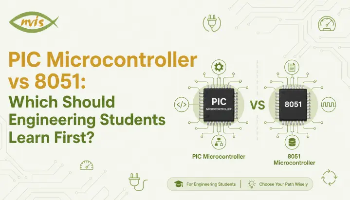
PIC Microcontroller vs 8051: Which Should Engineering Students Learn First?

Posted on 08-09-202608-09-2026 by Tushar Saluja

TL;DR

This blog is for ECE, EEE, and CSE engineering students, freshers, and GATE, SSC JE, and RRB JE aspirants who are confused about whether to start their embedded systems journey with a PIC microcontroller or 8051.
PIC refers to a family of Microchip microcontrollers, and many PIC families use RISC style instruction sets. The original 8051 architecture is generally classified as CISC. Both are still taught and used in Indian industry and exams today.
8051 is usually a better starting point academically because it exposes students to how memory, ports, and interrupts work at a very basic level, and it is a microcontroller most exam syllabi are built around.
PIC microcontrollers can be useful for hands-on hardware projects because many PIC devices integrate peripherals such as ADC, timers, PWM, and serial interfaces. However, industry uses many different MCU families, so students should also develop transferable skills in C, debugging, communication protocols, RTOS concepts, and modern MCU platforms.
The smartest strategy is not to pick one and ignore the other. Learn 8051 fundamentals for your exams and conceptual base, then move to PIC (or ARM based boards) for hands-on projects and placements.

All electronics students come to this crossroad at some point. You open your embedded systems lab book and it says, “8051 microcontroller.” You go to a hobbyist forum or placement group, and someone asks what a PIC microcontroller is used for, and swears by it for their final year project. Confusion really does come quickly.

One of the most frequent queries of engineering freshers entering into Embedded Systems is this one. PIC microcontroller and 8051 microcontroller are both popular, well documented and featured in Indian University syllabus as well as in competitive exams and job description. However, they have been constructed at different times, for different reasons, and to impart different knowledge.

This blog explains what PIC is in microcontroller terms, compares the two, and finally, which would be the first to pay attention to as a student. At the end of the day, you’ll have a firm, easy to understand solution rather than further puzzlement.

What Is a Microcontroller, in Plain English

Before comparing PIC and 8051, let’s get one basic idea straight, because a lot of students jump into comparisons without this foundation.

Think of a microcontroller like a tiny, dedicated employee inside a machine. It does not do everything a computer does. It does one job, and it does that job repeatedly and reliably. A microcontroller inside a washing machine only worries about spin cycles, water levels, and timers. It does not need to browse the internet or run a spreadsheet.

Technically, a microcontroller is a single chip that packs together a processor, memory, and input output circuitry, all in one place. Compare that to a microprocessor like one in your laptop, which needs separate memory chips and support circuitry to function. A microcontroller is self contained, like a mini computer built for one specific task.

Both PIC and 8051 fall under this “single chip mini computer” category. The difference lies in who designed them, how they process instructions, and how easy they are to work with.

What Is PIC Microcontroller, and Where Did It Come From

PIC is a family of microcontrollers developed by Microchip Technology. Many classic 8 bit PIC families use RISC style instruction sets, but PIC is a broad product family with different architectures and capabilities. In simple terms, RISC architectures generally use a relatively small set of streamlined instructions designed for efficient execution. The exact instruction cycle timing depends on the specific PIC family and device. Because many RISC architectures use a smaller set of relatively simple instructions, instruction execution can be efficient and predictable, although actual performance depends on the specific architecture and device.

Let’s get an analogy here to help make this sink in. Imagine two chefs. One chef (RISC, as PIC) knows a few basic cooking methods very well, and can mix them up quickly to come up with any dish. Another chef (CISC, 8051) has hundreds of special recipes – some of which require a few more steps to implement – because he does a lot in one. Both cooks are ‘correct’ but the first cook is more efficient at repetitive cooking jobs.

Many PIC microcontrollers use a Harvard style architecture in which program memory and data memory are accessed separately. Combined with instruction pipelining, this allows many instructions to be fetched and executed efficiently. This is why the PIC micros are capable of decent speed at lower clock frequencies.

Then what is a PIC Microcontroller used for in the real world? Its ease of development tools makes it suitable for a wide variety of consumer electronics such as remote controls and home electronics, industrial automation systems, automotive modules, and countless student and hobbyist projects. PIC devices are available across a wide range of performance and memory configurations, so the exact capabilities vary significantly between PIC families and individual models, making for a PIC variant that suits almost any project size, from a simple LED blinker to a reasonably sophisticated industrial controller.

What Is 8051, and Why Is It Still Taught Today

Intel developed 8051, an 8 bit microcontroller, back in 1981 and so it is more than 40 years old. So if you’re thinking, Why does a college still teach something this old in 2026? The honest answer is: it’s not about being modern; it’s about learning the fundamentals.

The 8051 is an 8 bit microcontroller with a CISC style instruction set. Continuing with the chef metaphor, this is a chef who can remember hundreds of recipes, some of which involve a number of steps to implement internally. Classic 8051 devices use a well defined machine cycle model, with individual instructions taking a specified number of machine cycles. PIC devices use a different instruction cycle model, so their timing should be compared on a device and instruction specific basis.

The real value of 8051 for the new programmer is the exposure of everything. The classic 8051 architecture includes internal program memory and RAM, while also supporting external program and data memory. This makes it useful for learning how a processor communicates with memory and peripherals at a relatively fundamental level. This is because when learning, it is possible to view how the processor communicates with the memory, rather than it all being hidden in the processor itself as it is in most modern microcontrollers. No compiler magic, no hidden pipeline behavior, and no mystery. You experience fundamentals.

That’s why 8051 still appears in many embedded-systems lab courses and exam-preparation materials in India. It teaches concepts and NOT conveniences.

Historically, 8051 based microcontrollers have been used in cost sensitive embedded applications and continue to appear in some legacy and simple control systems. Modern automotive and medical products, however, often use newer MCU architectures with more advanced safety, connectivity, and processing capabilities.

PIC vs 8051: Head to Head Comparison

Once you understand “why” behind each chip, actual technical differences become much easier to digest. Here is a side by side comparison covering what matters most for students.

Parameter	PIC Microcontroller	8051 Microcontroller
Developed by	Microchip Technology	Intel (1981)
Architecture type	RISC (Reduced Instruction Set)	CISC (Complex Instruction Set)
Memory architecture	Modified Harvard	Harvard (classic variants often use external memory)
Instruction set size	Around 35 instructions (PIC16 family)	Around 111 to 255 instructions depending on variant
Ease of programming	Easier for beginners, strong IDE support (MPLAB X)	Slightly steeper learning curve, relies on tools like Keil
Peripheral integration	Extensive: ADC, PWM, USB, CAN in higher end models	Basic peripherals: timers, UART, I/O ports
Power consumption	Generally lower, strong sleep modes	Moderate, varies heavily by manufacturer variant
Typical use in India	Hobby projects, industrial automation, consumer electronics	Academic labs, legacy industrial systems, exam syllabi
Best suited for	Real hardware projects, placements, prototyping	Building fundamental concepts, government exam prep

Notice that neither column says “better” outright. That’s intentional. The right choice depends entirely on what you are trying to achieve at this stage of your engineering journey.

A Worked Example: Comparing Instruction Execution

Numbers make this comparison much more concrete, and this is exactly the kind of question that shows up in exam vivas and GATE adjacent microcontroller papers.

Suppose you want to toggle an output pin, and both microcontrollers are running at a 12 MHz clock frequency.

On 8051: classic 8051 uses a machine cycle made up of 12 clock periods. So at 12 MHz, one machine cycle takes:

Machine cycle time = 12 divided by clock frequency = 12 divided by 12,000,000 Hz = 1 microsecond

Suppose we compare the instruction cycle timing of a classic 8051 and a PIC16 device, both using a 12 MHz oscillator. A classic 8051 machine cycle takes 12 oscillator periods, or 1 microsecond. A typical PIC16 instruction cycle takes 4 oscillator periods, or about 0.33 microseconds. However, the actual time required for a pin toggle operation depends on the specific instruction sequence and device.

On a PIC16 microcontroller: Most PIC16 instructions execute in a single instruction cycle, and one instruction cycle equals 4 clock periods (this is because PIC uses an internal clock divider). At same 12 MHz clock:

Instruction cycle time = 4 divided by 12,000,000 Hz = 0.33 microseconds approximately

At 12 MHz, a classic 8051 machine cycle is 1 µs because one machine cycle consists of 12 oscillator periods. A classic PIC16 instruction cycle is four oscillator periods, or approximately 0.33 µs. However, these are different timing units, so this comparison alone does not establish that one MCU is three times faster. The number of cycles required by the actual instruction sequence and the device’s peripheral architecture must also be considered.

This calculation shows why, for this particular instruction and clock frequency, a PIC16 can complete the operation in fewer instruction cycle periods than a classic 8051. It illustrates the difference in instruction cycle design, rather than proving that RISC always outperforms CISC.

Programming Experience: PIC vs 8051 for a Beginner

8051 uses a CISC architecture, or Complex Instruction Set Computing. Going back to our chef analogy, this is a chef with hundreds of recipes memorized, some of which take multiple steps internally to complete. That does not necessarily make it slower for every task, but its instruction timing differs from that of RISC-based devices such as many PIC microcontrollers.

What makes 8051 really useful to a beginner is that it’s very accessible. Classic 8051 devices include internal program memory and RAM while also providing mechanisms for accessing external program and data memory. This makes the memory interface particularly useful for learning how processors communicate with memory. PIC devices can be a good fit for products that benefit from integrated peripherals and an established development ecosystem, although the MCU family chosen ultimately depends on the product’s technical and commercial requirements. No magic compilers; no pipeline secrets; nothing mysterious here. You watch fundamentals happen.

This is precisely because 8051 continues to be used in embedded systems lab manuals, GATE related coursework, and government exam syllabus throughout India. It teaches principles, not conveniences.

In reality, 8051 based devices are more commonly associated with simple or legacy embedded applications, while newer automotive and medical systems generally use more modern microcontroller architectures.

India Context: Where These Microcontrollers Actually Matter

This is the part that most tutorials skip entirely, and it matters a lot if you are studying in India with placements or government exams in mind.

In many Indian engineering courses and some exam preparation materials, 8051 remains a commonly taught microcontroller because of its historical importance and simple architecture. For RRB JE Electronics & Allied Engineering, the current syllabus includes a broader “Microprocessor and Microcontroller” section covering microprocessors, assembly language programming, peripherals, other microprocessors, and microcontrollers. Candidates should therefore follow the latest official syllabus rather than assuming that every 8051 specific topic is explicitly prescribed. 8051 fundamentals can be useful if you are preparing for these exams, but candidates should prioritize the topics explicitly covered in the latest official syllabus.

The picture is wider on an industry and PSU level. ISRO, DRDO, and BEL employ electronics engineers for embedded systems roles involving areas such as satellite payloads, radar systems, and control systems. These roles usually require knowledge of microprocessors and microcontrollers, C programming, real time systems, and hardware interfacing rather than expertise in one specific MCU family. In the private sector, automotive Tier 1 companies, industrial automation firms, and IoT product companies use whichever microcontroller family fits their product needs, and PIC devices can be attractive in products where their integrated peripherals, memory options, package choices, and development ecosystem fit the design requirements.

Entry level embedded systems roles for freshers generally fall in 3 to 8 LPA range depending on company type and city, with service companies at lower end and product or automotive Tier 1 companies at higher end. Specializing more deeply within automotive embedded systems or IoT could take mid career packages further than this range as experience builds up. Bengaluru, Chennai, and Hyderabad are metropolitan cities with high demand for automobiles and semiconductors that provide better pay rates compared to other cities.

Practical implications for you as a student: 8051 can help you prepare for courses and exams that emphasize its architecture, while PIC or modern ARM based platforms such as STM32 can give you hands-on project experience. For placements, focus on transferable embedded systems skills rather than one specific microcontroller.

Exam Relevance: GATE, SSC JE, and RRB JE Strategy

If you are balancing coursework with competitive exam prep, here is how to prioritize your microcontroller study time.

For GATE ECE, note that microcontroller specific questions are not a dominant, separately weighted topic in official syllabus structure. GATE ECE leans heavily on Engineering Mathematics, Communications, Networks, and Signals and Systems, so microcontroller concepts usually surface indirectly through digital electronics and embedded logic questions rather than as a dedicated 8051 versus PIC comparison. Do not over invest your GATE prep time here at expense of higher weightage sections.

For SSC JE and RRB JE Electronics, the story flips completely. For exams where microcontroller architecture is explicitly included in the syllabus, candidates may encounter questions on areas such as 8051 architecture, addressing modes, timers, interrupts, and interfacing. Always use the latest official syllabus and previous year papers to determine the appropriate depth. If you are targeting these exams, treat 8051 syllabus as core preparation material, not optional reading.

For university semester exams and lab vivas, expect a mix. Many Indian engineering colleges still run their embedded systems lab entirely on 8051 kits, so practical viva questions will test your understanding of registers, timers, and interrupt handling on this chip specifically. If your final year project happens to use PIC or another RISC based microcontroller, be ready to explain architectural differences confidently since examiners often ask “why did you choose this over 8051.”

Career and Salary Outlook for Embedded Systems Engineers

Choosing between PIC and 8051 is really a small decision inside a much bigger career path: embedded systems engineering, and the outlook for this field in India remains genuinely strong.

Entry level embedded systems roles for freshers generally fall in 3 to 8 LPA range, with variation based on whether you join a service based company or a product focused firm. Automotive embedded roles involving areas such as AUTOSAR, CAN, and ADAS can offer strong career progression, particularly as engineers gain specialized experience. Once you gain a few years of specialized experience, mid-level engineers with 3 to 5 years of experience can move into the 8 to 14 LPA bracket, and senior embedded architects at larger semiconductor and automotive companies can cross well beyond that.

What actually drives these numbers upward is not which specific microcontroller you know, but how deep your fundamentals go combined with adjacent skills like RTOS concepts, embedded Linux, communication protocols such as I2C and SPI, and increasingly, IoT integration. A student who understands both 8051 fundamentals and modern PIC or ARM based development has a noticeably stronger foundation walking into interviews than someone who only memorized one chip’s datasheet.

India’s growing semiconductor push and EV manufacturing boom are also expanding demand for embedded talent significantly, which is good news if you are entering this field over the next few years.

So, Which Should You Learn First?

If you are a first or second year student building your foundation, or if you are preparing for SSC JE, RRB JE, or a university exam with 8051 in the syllabus, start with 8051. Its exposed architecture forces you to understand memory, registers, and interrupts at a level that pays off for years, even after you move to more modern chips.

If you are a third or final year student focused on projects and placements, consider moving beyond 8051 toward a modern MCU platform such as STM32, while also learning PIC if it aligns with your course, existing hardware, or project requirements, which are widely used across embedded, industrial, automotive, and IoT applications. PIC devices can also provide a useful bridge between academic microcontroller concepts and hands-on hardware development, particularly through the MPLAB X development environment and integrated peripherals.

The strongest students do not pick a side. They use 8051 to build conceptual depth, then use PIC (or ARM) to build practical, portfolio worthy projects. That combination is what actually gets noticed in interviews and technical rounds.

Conclusion

The PIC microcontroller vs 8051 debate is not really about which chip wins. It’s about matching the right tool to the right stage of your learning journey. 8051 hands you transparency and conceptual clarity, which is exactly what a beginner needs and exactly what Indian competitive exams still test. PIC microcontrollers can give you useful hands-on experience with peripherals, firmware development, and hardware interfacing. For broader placement preparation, however, combine that experience with C, communication protocols, debugging, RTOS concepts, and a modern MCU platform such as STM32.

Start with whichever your syllabus or exam demands right now, but make sure you eventually get comfortable with both. If you are just getting started, pick up an 8051 development kit or a PIC16F877A board, work through a few basic LED and interfacing projects, and build from there. That hands-on practice will teach you more in a weekend than any comparison article, including this one.

FAQs

: What is a PIC microcontroller used for in real projects?

PIC microcontrollers are used in consumer electronics like remote controls and home appliances, industrial automation systems, automotive control modules, and a large share of student and hobbyist electronics projects because of their beginner friendly MPLAB X toolchain and strong peripheral support.

What is PIC in microcontroller terminology, exactly?

PIC is the name used for a family of microcontrollers from Microchip Technology. The acronym is historically associated with ‘Peripheral Interface Controller,’ although the PIC family includes different architectures and capabilities. The name reflects its original design purpose of efficiently interfacing with external peripherals.

How do I start learning how to program a PIC microcontroller as a beginner?

Install MPLAB X IDE along with XC8 compiler, pick a common beginner friendly chip like PIC16F877A, connect a programmer such as a PICkit, and start with a simple LED blink project before moving on to interfacing sensors, displays, and motors.

Is 8051 still relevant, or should I skip straight to PIC or ARM?

8051 remains relevant for Indian academic syllabi, SSC JE and RRB JE exam preparation, and for building a strong conceptual foundation. Studying 8051 can provide a useful way to understand registers, memory access, interrupts, and low-level interfacing, particularly when those topics are part of your course or exam syllabus.

Which microcontroller is better for GATE preparation, PIC or 8051?

Neither carries heavy dedicated weightage in core GATE ECE syllabus, which focuses more on Communications, Networks, Signals and Systems, and Engineering Mathematics. Basic 8051 concepts occasionally support digital electronics and embedded logic questions, but this should not be a major focus area for GATE aspirants.

Can I directly learn PIC microcontroller without studying 8051 first?

Yes, it is technically possible, especially if your course or exam does not require 8051. However, many students find that skipping 8051 means missing out on foundational concepts around registers, addressing modes, and low level memory access, which are easier to grasp on 8051’s simpler, more transparent architecture.

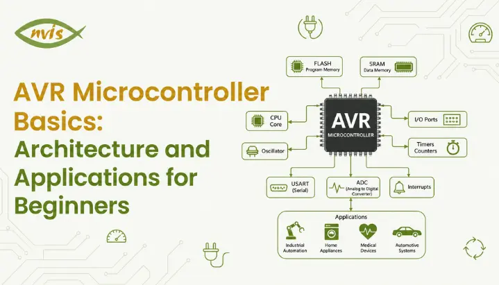
AVR Microcontroller Basics: Architecture and Applications for Beginners

Posted on 08-09-202611-09-2026 by Tushar Saluja

TL;DR

This blog is for ECE, EEE, and CSE students, embedded systems beginners, and GATE, SSC JE, and RRB JE aspirants who want a clear, practical understanding of AVR microcontrollers.
AVR is a family of 8-bit microcontrollers, with many classic AVR devices based on RISC and Harvard-style architectures and it is one of easiest and most widely taught microcontrollers in Indian engineering colleges.
This post breaks down what AVR microcontroller is, architecture of AVR microcontroller block by block, and where it is actually used in Indian industry.
You will also find a worked numerical example, a comparison with 8051, PIC, and ARM, and exam focused tips for GATE and SSC JE preparation.
By the end, you will know exactly why AVR is often the first microcontroller recommended for beginners, and how learning it can lead to real embedded systems career paths in India.

AVR is one of the best-known 8-bit microcontroller families, particularly in electronics education and hobbyist embedded development. It was developed by Alf-Egil Bogen and Vegard Wollan, and Atmel launched its first AVR devices in the late 1990s. The ATmega328P later became especially well known through the Arduino Uno platform. In this guide, we will cover what an AVR microcontroller is, how its architecture works, how its concepts relate to competitive-exam preparation, and how these fundamentals connect to a career in embedded systems.

What is AVR in a Microcontroller?

A microcontroller is a little, self contained computer that fits on one chip. It doesn’t require a separate keyboard, monitor or hard drive as all the components it requires – processor, memory, and input output – are built in.

Suppose you would like to use this little computer to blink an LED, read the temperature of a sensor, or control a motor in a washing machine. That’s what a microcontroller’s job is all about! Does not attempt to open a Web browser or play videos. Designed to perform one specific task efficiently, consistently, repeatedly, and often for years without a problem.

What is an AVR microcontroller, then? AVR is a series of 8 bit microcontrollers that are based upon the Reduced Instruction Set Computing (RISC) architecture. RISC stands for the fact that the chip will know a few simple instructions, and will execute most of them in just one clock cycle rather than multiple, as was the case with the older designs. This is one reason AVR is classified as an 8-bit microcontroller family: its core architecture is designed around 8-bit data operations.

AVR microcontroller was developed by two students at Norwegian Institute of Technology, Alf Egil Bogen and Vegard Wollan. In 1997, Atmel bought the design and produced the first commercial AVR chip, AT90S1200. The name AVR is commonly associated with the initials of its original designers, Alf-Egil Bogen and Vegard Wollan. ‘Advanced Virtual RISC’ is sometimes given as an expansion, but it is not generally treated as the official meaning of AVR.

Arduinos use an AVR microcontroller, so if you have ever used an Arduino Uno, you have already used an AVR microcontroller. That chip, ATmega328P, is a good old microcontroller, which is one reason AVR has become a familiar entry point for many students learning embedded systems through Arduino-based projects.

Architecture of AVR Microcontroller Explained Simply

Think of a little factory, before you get into the technical blocks. The raw material enters via one gate, the finished goods exit via another, and the instruction is fed from the factory’s rule book via a third. No confusion in the streets as each type of traffic runs on its own road.

For a deeper look at AVR’s CPU core, registers, pipelining, and Harvard architecture, see Microchip’s AVR CPU Core documentation, in which program memory and data memory have separate buses. This is in contrast to most desktop computers that have von Neumann architecture, which involves both instructions and data sharing the same bus. AVR uses separate program and data memories and buses. Its CPU also uses a simple instruction pipeline, allowing the next instruction to be fetched while the current instruction is being executed and it’s one of the main reasons AVR chips can perform almost 1 instruction per clock cycle.

Let’s go through the essential components of AVR microcontrollers, one by one.

CPU Core and General Purpose Registers

The CPU core is at the core of any AVR chip, which is then tied to 32 general purpose 8-bit-wide registers. That’s quite a whopping amount for an 8 bit microcontroller. Microchip provides a detailed explanation of the AVR’s 32 general-purpose registers compared with many earlier 8-bit microcontrollers, reducing the need to fetch data from slower memory as often.

These 32 registers are closely integrated with the AVR CPU core, allowing instructions to access registers efficiently. Many AVR instructions can read operands from the register file and write the result back within a single instruction cycle. This register organization can reduce the need for frequent memory accesses and contributes to efficient instruction execution.

Memory Organization

The AVR microcontrollers control three different types of memory and each has a distinct purpose.

The actual program code is stored in flash memory. Flash memory is non-volatile, so it retains the program when power is removed. It can be erased and reprogrammed many times, including through In-System Programming (ISP) on supported AVR devices. This allows supported AVR devices, including the ATmega328P used in classic Arduino Uno boards, to be reprogrammed repeatedly within the device’s specified write-cycle limits.

SRAM or Static Random Access Memory: Memory used for temporary data during the execution of your program, e.g., variable values and stack. SRAM is volatile, meaning that it loses its contents when the power is removed, unlike flash.

EEPROM is a smaller portion of non volatile memory that is used to hold data that remains even after a power down, such as calibration values or a saved setting for a configuration. As an example, if you’re designing an electronic door lock, access code could be stored in EEPROM and therefore it will not be lost if the device is disconnected.

ALU and Single Cycle Execution

Actual number crunching takes place in the Arithmetic Logic Unit, where addition, subtraction, logical comparisons, bit manipulation occur. The ALU is located next to 32 general purpose registers, so most AVR instructions run in one clock cycle.

That is precisely why AVR feels ‘snappy’ when compared to older 8 bit designs requiring more than 1 clock cycle an instruction. For instructions that execute in a single clock cycle, a 1 MHz AVR can theoretically execute up to about 1 million instructions per second. The higher the clock the higher the throughput, at the expense of increased power consumption.

I/O Ports, Timers, and Peripherals

The surrounding CPU core is a set of peripherals that let the microcontroller talk to the outside world. AVR chips typically expose their pins as 8 bit I/O ports, commonly labelled Port A, Port B, Port C, and Port D depending on specific chip. Each port can be configured pin by pin as either input or output.

On top of basic I/O, AVR microcontrollers include built in timers and counters, an Analog to Digital Converter or ADC for reading analog sensor signals, communication interfaces like USART, SPI, and I2C for talking to other chips, and a watchdog timer that automatically resets microcontroller if program ever gets stuck in an infinite loop. There is also an interrupt controller, which allows the chip to instantly pause its current task and respond to an urgent event, like a button press, without constantly checking for it in a slow polling loop.

Worked Numerical Example: Calculating Execution Time

Understanding the relationship between clock frequency, instruction cycles, and execution time is useful for microprocessor and microcontroller exam preparation. Here is a simple worked example using AVR’s single cycle execution model.

Problem: An AVR microcontroller operates at a clock frequency of 8 MHz. Assuming most instructions execute in a single clock cycle, calculate time taken to execute one instruction and number of instructions executed in one second.

Step 1: Find clock period. Clock period T equals 1 divided by frequency. T = 1 / (8 x 10^6 Hz) = 0.125 microseconds per cycle.

Step 2: Since most AVR instructions take one clock cycle, execution time per instruction is approximately 0.125 microseconds.

Step 3: Calculate instructions per second. For the simplified assumption that each instruction takes one clock cycle, the theoretical instruction throughput is approximately equal to the clock frequency: 8 million instructions per second, or 8 MIPS.

Interpretation: This is why AVR datasheets often state performance directly in MIPS at a given clock frequency. Compare this with classic 8051 implementations, which commonly use 12 oscillator periods per machine cycle, although newer 8051-compatible devices can use fewer cycles. A classic 12-clock 8051 requires 12 oscillator periods for a machine cycle, so an 8 MHz clock corresponds to about 666,667 machine cycles per second. However, actual instructions can require different numbers of machine cycles, so this should not be treated as a direct instruction-per-second comparison with AVR. This single comparison is a favorite in exam numericals because it tests both your formula knowledge and your conceptual understanding of RISC versus CISC design.

AVR vs 8051 vs PIC vs ARM: How Do They Compare?

Students preparing for interviews or exams are frequently asked to compare AVR with other microcontroller families. Here is how they stack up on fundamentals that matter most.

Feature	AVR	8051	PIC	ARM Cortex M
Architecture	RISC, Harvard	CISC, Von Neumann	RISC, Harvard	RISC, Harvard
Data width	8 bit	8 bit	8/16 bit	32 bit
Cycles per instruction	Mostly 1	12 (classic), 1 (enhanced)	Mostly 1 to 4	Mostly 1
General purpose registers	32	Limited (accumulator based)	Fewer, banked registers	13 general registers
Typical use case	Hobby projects, mid range embedded control	Legacy industrial systems, teaching	Motor control, automotive	IoT, smartphones, complex embedded systems
Beginner friendliness	High, Arduino ecosystem	Moderate, widely taught in colleges	Moderate	Lower, steeper learning curve

AVR sits in a comfortable middle ground. Its register organization and instruction model can make AVR easier for many beginners to work with than classic 8051 implementations, while ARM Cortex-M devices offer substantially greater processing capability for more demanding applications. This balance makes AVR a useful starting point before moving to more advanced ARM-based development, particularly Cortex-M platforms used widely in IoT, automotive, industrial automation, and other embedded applications.

Real World Applications of AVR Microcontroller

AVR microcontrollers are not confined to college labs. AVR microcontrollers have been used across consumer electronics, industrial control, instrumentation, automotive subsystems, and hobbyist projects, although the specific devices selected in modern products vary widely by application.

AVR devices have been used in consumer electronics, home automation, instrumentation, and other control applications, although the specific MCU used in a commercial product depends on its technical requirements. AVR based modules handle tasks like dashboard indicators and basic sensor monitoring, though more complex modern vehicle systems increasingly rely on 32 bit processors.

Robotics and drone hobby projects frequently use AVR based boards for tasks like motor control, sensor fusion at a basic level, and communication between subsystems. AVR microcontrollers can also be useful for low-complexity monitoring, control, and instrumentation prototypes. AVR also plays a strong role in industrial signal sensing, data acquisition systems, and prototyping new hardware designs before a company commits to a more expensive custom chip.

Perhaps the biggest reason for AVR’s popularity, though, is education. Because classic Arduino boards such as the Uno R3 use AVR microcontrollers, the Arduino ecosystem has helped introduce many students and hobbyists to AVR-based embedded development, including a huge number of Indian engineering students, to get their first hands on experience with embedded systems.

AVR Microcontroller in Indian Engineering and Job Market Context

For Indian engineering students, AVR is more than an academic topic. It connects directly to real employment opportunities and government backed industry growth.

Organizations such as ISRO, DRDO, BEL, and BHEL recruit engineers for electronics, embedded systems, control, instrumentation, and related roles. The specific microcontroller or processor technologies used vary by project, so students should view AVR as a foundation for embedded-systems concepts rather than as a guaranteed technology used by these organizations. Private sector opportunities are expanding quickly too, driven by India’s growing semiconductor and electronics manufacturing push. India’s semiconductor and electronics ecosystem is also receiving policy support, with initiatives focused on domestic manufacturing, semiconductor development, research, and workforce development. India has a significant share of the global semiconductor design workforce, according to Indian government and industry estimates, which means AVR can provide a foundation in registers, memory, peripherals, interrupts, and firmware development. These fundamentals can then support further specialization in embedded software, firmware, verification, semiconductor design, or other electronics roles.

Government initiatives such as the Production Linked Incentive (PLI) schemes and broader electronics-manufacturing policies are supporting investment and capacity growth in India’s electronics ecosystem. This growth can create additional opportunities for engineers with embedded-hardware and firmware skills. This growth can create opportunities for engineers with embedded hardware and firmware skills. Learning AVR can provide a foundation in registers, memory, peripherals, interrupts, and firmware development that can be transferred to other MCU platforms.

For students targeting the EV sector, embedded controllers in Battery Management Systems and motor drive units often build on the same fundamental microcontroller concepts covered here, even when the specific chip used is a more advanced ARM based part.

GATE, SSC JE, and RRB JE Exam Relevance

Microprocessor and microcontroller concepts appear in relevant engineering and technical-exam syllabi, although the exact topics and weightage vary by exam and year, so it is worth preparing strategically rather than memorizing randomly.

For GATE EC preparation, concepts such as machine instructions and addressing modes, ALU, data paths and control, and instruction pipelining are covered under Computer Organization. AVR-specific details are not required by the GATE EC syllabus. For GATE IN and other papers, the relevant topics depend on the current official syllabus for that specific paper. AVR-specific details should therefore be treated as a way to strengthen fundamentals rather than as a guaranteed GATE topic. For technical recruitment exams that include electronics or microprocessor/microcontroller topics, focus on fundamentals such as microprocessor operation, memory, digital electronics, and interfacing. Always check the latest official syllabus for the specific exam and post.

A smart strategy is to master fundamental concepts, RISC versus CISC, Harvard versus Von Neumann architecture, register organization, and memory types, since these concepts repeat across multiple microcontroller families in syllabus, not just AVR. Once you are comfortable with AVR’s architecture, understanding 8051 or PIC becomes significantly easier because underlying principles overlap heavily.

Solving previous-year papers that cover microprocessor, microcontroller, and digital-electronics concepts is a useful way to prepare, particularly because the question style and emphasis can vary between exams and recruitment cycles, since these questions test the same clock cycle and MIPS calculation pattern shown earlier in this post, just with different numbers.

Career and Salary Outlook for Embedded Systems Engineers in India

Embedded systems is an important career path within electronics and electrical engineering in India, and microcontroller knowledge is one of the foundational skills for entering the field.

Freshers entering embedded systems roles in 2026 can typically expect salaries in the range of roughly 3 to 8 LPA, depending on their skill set, internship experience, and project portfolio. Freshers specifically at automotive Tier 1 companies and semiconductor firms often start around 4 to 8 LPA, while service based companies tend to offer figures at lower end of typical fresher ranges. As experience grows, compensation rises meaningfully. Professionals with three to five years of experience can expect roughly 8 to 14 LPA on average, and senior embedded architects at major companies can reach 20 to 38 LPA.

Skills that meaningfully boost these numbers include familiarity with multiple microcontroller families such as ARM Cortex, PIC, and AVR, exposure to Real Time Operating Systems like FreeRTOS, and domain specialization in automotive or IoT embedded systems. Building two or three solid personal projects using an AVR based board like Arduino, then progressing to STM32 or another ARM based platform, is a practical and low cost way for students to build a portfolio that stands out during placements.

Conclusion

AVR microcontroller remains one of best entry points into embedded systems for engineering students in India, and for good reason. Its RISC-based instruction model, register-rich architecture, and generally efficient instruction execution make it a useful platform for learning embedded-systems fundamentals. From understanding what an AVR microcontroller is and breaking down its architecture, to solving exam style numericals and mapping out real career paths, this post has covered the complete picture a student needs.

If you are preparing for GATE, SSC JE, or RRB JE, treat AVR as your foundation rather than an isolated topic. The concepts you learn here RISC versus CISC, memory organization, register-based execution, and instruction timing carry over to 8051, PIC, ARM, and other microcontroller platforms. And if you are exploring embedded systems as a career, pick up an AVR based board like Arduino, build a few small projects, and use that hands-on experience as your first real step toward a career in India’s rapidly growing electronics and semiconductor industry.

Frequently Asked Questions

What is AVR in microcontroller terms, in one line?

AVR is a family of 8-bit microcontrollers associated with RISC-based and Harvard-style architectures, with many classic AVR devices supporting efficient single-cycle instruction execution and widespread use in devices like Arduino boards.

What AVR microcontroller is used by beginners specifically?

A common beginner platform is the ATmega328P, which is used in the classic Arduino Uno. Other AVR devices are also used in development boards and standalone projects to learn programming fundamentals, build simple LED and sensor projects, and understand core embedded systems concepts before moving to more advanced platforms.

Is the architecture of AVR microcontrollers difficult to learn compared to 8051?

AVR can be easier for many students to grasp because of its relatively straightforward instruction model and register organization, although the difficulty depends on the student’s background and the specific AVR device being studied even though 8051 is often taught first in many Indian college syllabi.

Does AVR microcontroller training help with GATE or SSC JE preparation?

Yes, AVR can help students understand general microcontroller concepts such as registers, memory, instruction execution, and peripherals. However, students should prepare according to the current syllabus of each examination rather than assuming AVR-specific knowledge is required.

What is the difference between AVR and ARM microcontrollers?

AVR is an 8 bit microcontroller family suited for simpler, cost sensitive applications, while ARM Cortex M microcontrollers are 32 bit and handle more complex, memory intensive, and connectivity heavy applications like IoT devices and modern automotive systems.

Can learning AVR microcontroller basics lead to a good embedded systems career in India?

Yes, AVR is widely used as a foundational learning platform, and skills it builds directly support entry into embedded systems roles in India, where entry-level salaries vary considerably depending on the employer, location, skills, and project experience.

Three Phase AC Voltage Controller Waveforms Explained: Modes, Working and Applications

Posted on 15-08-202615-08-2026 by Tushar Saluja

TL;DR

This blog is for electrical and electronics engineering students, freshers, and GATE, SSC JE, and RRB JE aspirants who want a clear, practical understanding of three phase AC voltage controller waveforms.
A three phase AC voltage controller uses six thyristors to control RMS voltage delivered to a three phase load without changing supply frequency.
output waveform depends on firing angle alpha, which falls into three distinct conduction modes, each producing a different chopped voltage shape.
A worked numerical example ties waveform theory to real RMS voltage and power calculations that students can reproduce in exams and labs.
The topic carries real weight in GATE Power Electronics and in India’s growing power electronics, EV, and industrial automation job market.

A three phase AC voltage controller is a circuit that controls the RMS value (effective value) of AC voltage supplied to a three phase load without changing the supply frequency. It uses six thyristors, two connected in anti parallel per phase, fired at a controlled delay angle after each natural commutation point. This blog explains how circuit operates, breaks down three conduction modes that shape its output waveforms, and connects theory to Indian industry applications, GATE exam relevance, and career paths in power electronics.

What Is a Three Phase AC Voltage Controller

Think about a fan regulator in your home. When you turn the knob, you are not changing the frequency of the AC supply coming into your house. You are simply controlling how much of each voltage cycle actually reaches the fan motor. Turn it down, and the fan gets a smaller “slice” of each cycle. Turn it up, and it gets more.

A three phase AC voltage controller does exactly this, but at an industrial scale, across three phases simultaneously, and using thyristors instead of a mechanical knob. Instead of a ceiling fan, load could be a large induction motor, an industrial heater bank, or a set of high power lamps drawing current from a three phase supply.

The main idea is simple. The controller does not convert AC into DC. It works only with AC and controls how much voltage reaches the load. It just “chops” each half cycle of input waveform, letting through only a controlled portion of it, so RMS voltage reaching load can be adjusted smoothly from close to full supply voltage down to nearly zero.

Because it controls AC voltage without changing it into DC, this circuit is also called an AC-to-AC converter or an AC voltage regulator. The primary keyword here, three phase AC voltage controller, refers to this exact family of circuits, and understanding its waveform behavior is the foundation for everything else in this topic.

How Circuit Works: Thyristors, Firing Angle and Natural Commutation Point

Before learning the waveforms, you should understand three basic ideas: a thyristor pair, the firing angle, and the natural commutation point.

Each phase of the controller uses two thyristors connected back to back, or antiparallel. One thyristor conducts during the positive half cycle of that phase’s voltage, and the other conducts during the negative half cycle. This antiparallel pairing is necessary because a single thyristor can only conduct current in one direction, but an AC load needs current flowing both ways across a full cycle.

A natural commutation point is the moment when one thyristor turns off and another takes over because the AC supply changes direction. It serves as the reference point from which the firing angle is measured. For a three phase system, this point repeats every 60 degrees because there are six such transitions in every 360 degree cycle, one for each thyristor.

The firing angle (α) is the delay between the natural commutation point and the moment the thyristor is switched on. If alpha is small, thyristor turns on almost as soon as it is able to, and load receives nearly full voltage. If alpha is large, thyristor turns on late in cycle, so it conducts for a shorter time, and load receives a smaller RMS voltage.

Two more terms matter here. A thyristor turns off automatically the moment its current falls to zero, which is called natural or line commutation. And for a thyristor to actually fire, two conditions must be true at the same time: its anode voltage must be higher than its cathode voltage, and a gate pulse must be present. Instead of sending one short gate pulse, engineers often send several pulses over a short period. This makes sure the thyristor turns on even if the exact switching time changes slightly and a single narrow pulse might be missed.

Three Phase AC Voltage Controller Waveforms: Mode I, II and III Explained

This is the most important part of the topic. Many textbooks become difficult here because they start with maths instead of explaining the idea first. Before math, picture what is physically happening: as you increase firing angle alpha, fewer thyristors are conducting at any given instant, and shape of chopped waveform changes character three distinct times. Power electronics engineers label these three characters Mode I, Mode II, and Mode III.

Mode I: 0° ≤ α < 60°

In this range, the controller behaves almost like an uncontrolled circuit. At any instant, either two or three thyristors are conducting simultaneously. Because nearly full waveform gets through, output closely resembles undelayed sine waves, only slightly clipped near the start of each half cycle. This mode delivers the highest RMS output voltage range, from full supply voltage down to roughly 96 to 97 percent of it as alpha approaches 60 degrees.

Mode II: 60° ≤ α < 90°

Here behavior changes noticeably. At any given moment, exactly two thyristors conduct, one from each of two different phases. There is no longer a window where three thyristors conduct together. The output waveform now has small gaps where the voltage becomes zero before the next thyristor turns on. This is the transition zone where the chopped nature of the waveform becomes visually obvious on an oscilloscope.

Mode III: 90° ≤ α < 150°

In this final mode, the thyristors do not conduct continuously. There are short periods when no current flows. Sometimes two thyristors conduct together, and sometimes none conduct at all, leaving load voltage at zero for stretches of cycle. output RMS voltage drops sharply through this range, falling from around 70 percent of supply voltage at alpha equals 90 degrees to nearly zero as alpha approaches 150 degrees, which is the theoretical extinction point for a purely resistive star connected load.

Worked Numerical Example

Suppose a three phase, star connected, three wire AC voltage controller supplies a balanced resistive load with R equal to 10 ohms, connected to a 380 volt line to line, 50 Hz supply, and firing angle alpha is set to 30 degrees.

Since α = 30° is in Mode I, almost the full supply voltage reaches the load. Phase voltage Vm here corresponds to a line to neutral RMS value of about 220 volts. At alpha equals 30 degrees, standard control characteristic tables for this configuration show output RMS phase voltage is close to 98.5 percent of supply phase voltage, giving an output of roughly 216 to 217 volts RMS per phase.

Using this output voltage, RMS load current per phase works out to approximately Vo,rms divided by R, and output power per phase follows from Vo,rms squared divided by R. For a balanced three phase load, total output power is simply three times per phase power. This is exactly the kind of calculation that appears in GATE and university exam papers, so working through it by hand, rather than only reading derivation, builds real exam readiness.

Now compare this to alpha equals 90 degrees on the same circuit. System shifts into Mode III, and output RMS voltage collapses to roughly 70 percent of supply value, which more than halves delivered power compared to alpha equals 30 degrees, since power scales with square of voltage.

Comparison Table: Single Phase vs Three Phase AC Voltage Controller

Parameter	Single Phase AC Voltage Controller	Three Phase AC Voltage Controller
Thyristors required	2 (one antiparallel pair)	6 (two per phase)
Firing angle range for full control	0° to 180°	0° to 150° for resistive star load
Number of conduction modes	Not applicable	Three distinct modes (I, II, III)
Typical applications	Lamp dimming, single phase heaters, small fan regulators	Three phase motor speed control, industrial heaters, soft starters
Harmonic content	Odd harmonics present	Odd harmonics present, triplen harmonics depend on connection type
Control complexity	Simple, single firing circuit	More complex, six coordinated firing circuits
Common connection types	Direct or with transformer	Star three wire, star four wire, or delta connected

Applications of Three Phase AC Voltage Controller in Industry

Three phase AC voltage controllers are used in industries where AC power needs to be controlled smoothly without converting it into DC. The most common application is limited speed control of induction motors, mainly in fan and pump applications where torque requirements permit voltage control used in fans, pumps, and conveyor systems, where the controller adjusts voltage fed to the stator to vary motor speed and torque within limits.

Industrial heating systems are another major use case, particularly in furnaces and ovens where precise temperature control depends on regulating RMS voltage delivered to heating elements rather than switching them fully on or off. Static VAR compensators and soft starters for large motors also rely on the same underlying phase control principle, using controlled firing of thyristors to limit inrush current during motor startup.

Lighting control for large scale industrial or commercial installations, where dimming needs to happen uniformly across all three phases, is a further application area, along with certain classes of certain thyristor-based AC voltage regulators used in industrial power control with sensitive equipment.

India Context: Industry, Employers and Regulatory Landscape

In India, three phase AC voltage controllers and a broader family of AC to AC power electronic converters are core building blocks in sectors that the government has been actively pushing: renewable energy integration, industrial automation, and electric mobility. Companies such as BHEL, L&T, Siemens, ABB, and Crompton Greaves design and manufacture equipment that relies on this class of thyristor based control, particularly for motor drives and industrial power quality equipment.

Government policies also play an important role. Bureau of Energy Efficiency and broader push toward energy efficient industrial motors under India’s national programs have increased demand for engineers who understand voltage and speed control at power electronics level, not just at mechanical or control systems level. As India’s manufacturing sector modernizes under initiatives like Make in India and Production Linked Incentive schemes for electronics and semiconductor manufacturing, practical skill of reading and designing around thyristor controlled AC waveforms remains directly employable.

Public sector undertakings such as NTPC, PowerGrid, and BHEL, along with private players expanding into EV charging infrastructure and grid scale power electronics, continue to hire electrical engineers with a solid grounding in power electronics fundamentals, of which three phase AC voltage controller is a standard part of undergraduate and GATE syllabus.

Career and Salary Guidance in Power Electronics (India, 2026)

The average salary for a Power Electronics Engineer in India currently stands close to eight lakh rupees per year, with a typical range roughly between five and a half lakhs and eleven and a half lakhs annually depending on experience and employer. At fresher level, entry into government and PSU roles through GATE typically corresponds to a fixed pay scale in the six to twelve lakh range, while private sector roles in EV and semiconductor adjacent power electronics work can pay significantly more once a few years of hands-on experience are added.

Engineers who learn power electronics, motor drives, and battery management systems usually have better career opportunities for EV and grid integration space are seeing some of the fastest salary growth in the Indian market right now, with experienced roles in this niche commanding substantially higher packages than generalist electrical engineering positions. Renewable energy, industrial automation with PLC and SCADA skills, and defence and aerospace power systems roles round out strongest career tracks for someone who has built a genuine understanding of AC voltage control and related power conversion topics.

For students planning their career path, practical advice is straightforward: a strong grip on power electronics fundamentals such as three phase AC voltage controller, combined with hands on simulation experience using tools like MATLAB or PSIM, and a competitive GATE score, opens doors to both well established PSU route and faster growing private sector opportunities in EV and renewable energy companies.

GATE / SSC JE / RRB JE Exam Relevance

Power Electronics is one of higher weightage sections in GATE Electrical Engineering paper, and AC voltage controllers fall squarely within its syllabus alongside rectifiers, choppers, and inverters. Questions on this topic typically test three things: ability to identify correct conduction mode for a given firing angle, ability to compute RMS output voltage or output power for a stated alpha, and conceptual understanding of thyristor firing and commutation.

For SSC JE and RRB JE aspirants, depth of numerical analysis expected is usually lower than GATE, but conceptual questions on thyristor operation, purpose of firing angle, and basic difference between single phase and three phase AC voltage controllers appear regularly in power electronics and basic electrical engineering sections of these exams.

For exams, first learn the three conduction modes and their firing angle ranges. Many questions can be answered by identifying the correct mode and their alpha ranges first, since a large share of objective questions can be answered correctly just by recognizing which mode a given firing angle falls into, without needing to solve full RMS voltage integral under exam time pressure.

Conclusion

A three phase AC voltage controller regulates AC power the same way a fan regulator does, just scaled up to industrial three phase loads using six coordinated thyristors instead of a single mechanical dial. The output waveform passes through three distinct conduction modes as firing angle alpha increases from 0 to 150 degrees, and recognizing these modes is key skill for both exam problems and real circuit analysis. This topic is important because it is asked in GATE exams and is also widely used in industry in India’s growing power electronics, EV, and industrial automation sectors, which makes it worth mastering properly rather than memorizing formulas. Work through worked examples in this blog on paper, try varying firing angles yourself, and you will find underlying logic becomes intuitive far faster than equations alone suggest.

FAQs

What is the difference between a three phase AC voltage controller and a rectifier?

A rectifier converts AC input into DC output, while a three phase AC voltage controller keeps output in AC form and only adjusts its RMS magnitude. Both use thyristors and firing angle control, but the controller never creates a DC link.

Why does a three phase AC voltage controller need six thyristors?

Each of three phases needs an antiparallel pair of thyristors to handle both positive and negative half cycles of that phase’s voltage, since a single thyristor conducts in only one direction. Three phases multiplied by two thyristors each gives six total.

What are three modes in three phase AC voltage controller waveforms?

Mode I covers firing angles from 0 to 60 degrees where two or three thyristors conduct together, Mode II covers 60 to 90 degrees where exactly two thyristors conduct at a time, and Mode III covers 90 to 150 degrees where conduction becomes intermittent and can drop to zero.

What is the maximum firing angle for a three phase full wave AC voltage controller with resistive load?

For a star connected three wire configuration with a balanced resistive load, practical extinction point is around 150 degrees, beyond which output voltage effectively falls to zero.

Is three phase AC voltage controller topic important for GATE Electrical Engineering?

Yes, it falls under Power Electronics section of GATE EE syllabus, which typically carries significant weightage, and questions frequently test conduction mode identification and RMS output voltage calculations.

Where are three phase AC voltage controllers used in Indian industry?

They are commonly used for three phase induction motor speed control, industrial heating and furnace applications, soft starters for large motors, and certain lighting and power quality applications in manufacturing plants across companies like BHEL, L&T, Siemens, and ABB.

Sumpner’s Test of Transformer: Working Principle, Circuit, and Procedure Explained

Posted on 01-08-202601-08-2026 by Tushar Saluja

TL;DR

This blog is for engineering students, freshers, and anyone preparing for GATE, SSC JE, RRB JE, or discom JE exams who wants to actually understand Sumpner’s test, not just memorize it.
Sumpner’s test (also called back to back test) lets you find a transformer’s iron loss and copper loss together, at full load, without connecting any real load to it.
It works by connecting two identical transformers so their secondaries cancel each other’s voltage, which tricks the system into simulating full load current while actual power drawn from supply stays tiny.
Two wattmeters do real work here one reads combined iron loss, other reads combined copper loss at full load, and a simple worked example later in this blog shows exactly how those numbers turn into efficiency and voltage regulation.
With India adding record transformer capacity through grid expansion projects in 2026, understanding this test isn’t just exam prep, it’s a real skill that shows up in testing labs at BHEL, POWERGRID, Siemens India, and CG Power.

Picture two friends trying to test how much weight a bridge can hold. Building a full scale replica bridge and loading trucks onto it would work, but it would cost a fortune and waste a huge amount of material just for one test. Now imagine there was a clever way to simulate the exact same stress on a bridge, using almost no material at all. That is essentially what Sumpner’s test does for transformers.

Sumpner’s test, also known as back to back test, is a method used to determine efficiency, voltage regulation, and heating behavior of a transformer under full load conditions, without ever connecting a real load to it. It solves a problem that has bothered electrical engineers for over a century: how do you test something as large as a power transformer at full load, when arranging that load in real life is expensive, wasteful, and sometimes just not possible.

This blog breaks concepts down from scratch. You will learn why this test exists, how circuit is set up, why physics behind it actually works, how to calculate efficiency and regulation from real readings, and why this topic still matters heavily in 2026, both for competitive exams and for real jobs in India’s fast growing power sector.

Why Do We Even Need a Test Like This?

Before understanding Sumpner’s test, it helps to understand the problem it was built to solve.

Every transformer loses some energy while it works. This loss shows up as heat, and it comes from two sources. First is iron loss (also called core loss), which happens inside a transformer’s core simply because it is carrying a changing magnetic field, whether or not any load is connected. Second is copper loss, which happens in windings because current flowing through wire generates heat, and this loss grows as load increases.

To measure these losses individually, engineers normally use two simpler tests: open circuit (OC) test and short circuit (SC) test. OC test gives you iron loss, and SC test gives you copper loss. Between two, you get a complete picture of the transformer’s equivalent circuit.

Here is the catch. In real operation, a transformer does not experience iron loss and copper loss separately. It experiences both at same time, continuously, while carrying its actual load. So while OC and SC tests are great for calculating losses on paper, they cannot tell you how hot a transformer will actually get when it is running under genuine full load for hours. That missing piece is temperature rise, and it matters enormously for large transformers, because overheating is one of fastest ways to damage insulation and shorten a transformer’s life.

So the real question becomes this: how do you load a transformer to its full rated capacity, long enough to observe realistic heating, without burning through massive amounts of electricity on an artificial load? This is exactly the gap that Sumpner’s test fills.

Core Idea: Making Two Transformers Load Each Other

Here is where analogy becomes useful again. Instead of using one giant external load to stress test a transformer, what if you could make two identical transformers push against each other, so that one effectively becomes a load for the other?

That is precisely the trick behind Sumpner’s test. It is sometimes even called regenerative test, because most of the power circulating between two transformers gets returned to the system rather than wasted, similar to how two people arm wrestling exert real force on each other without needing a third person to push against them from outside.

For this test to work, you need two transformers that are identical in rating, turns ratio, and impedance. This is a genuine limitation, since not every lab or testing facility has two matching transformers available, especially for large custom built power transformers. But wherever this condition can be met, the payoff is huge: you get a full load test using only a small fraction of actual full load power.

How Circuit Is Actually Connected

Now let’s get into wiring itself, one step at a time, because this is where most explanations jump too fast.

Take two identical transformers, call them T1 and T2. Their primary windings are connected in parallel and connected directly to normal rated supply voltage and frequency, exactly as they would be in real operation. So far, this is nothing unusual.

An interesting part happens on the secondary side. secondary windings of T1 and T2 are connected in series, but with their polarities deliberately opposed to each other. In plain terms, voltage induced in one secondary winding is arranged to cancel out voltage induced in another.

Since both transformers are identical, their induced secondary voltages are equal in magnitude. When you connect them in opposition, those two equal and opposite voltages cancel each other out almost perfectly. net voltage around that secondary loop becomes zero.

Before starting the test, this connection has to be verified. Engineers do this by taking two secondary terminals and joining them together, then measuring voltage across the remaining two terminals with a voltmeter. If that voltmeter reads zero, secondaries are correctly connected in phase opposition, and setup is ready. If voltmeter instead reads a value close to double rated secondary voltage, it means connections are wrong and need to be reversed.

Two wattmeters are placed into this circuit to do actual measuring. One wattmeter sits on the primary side and records power drawn from the main supply. A second wattmeter is placed in the secondary loop, and it comes into play once an additional small voltage is deliberately injected into that loop using a low voltage regulating transformer or auto transformer.

Why Secondary Voltage Cancels Out (Physics Behind It)

It is worth pausing here, because most resources simply state that secondary voltages cancel without really explaining why that matters.

When primaries are energized and secondaries are left open (before any voltage is injected), a small no load current flows in each primary winding. This current exists purely to set up magnetic flux in each core and to supply core’s iron losses. Since two transformers are identical, this no load current is the same in both.

Because secondary voltages are equal and opposite, no current flows around the secondary loop at this stage. This means the secondary is effectively acting as an open circuit, even though it is physically a closed loop. In other words, this initial condition is quietly simulating the exact same situation as an open circuit test, just using two transformers instead of one.

wattmeter on the primary side, at this stage, is reading power needed to supply combined iron losses of both transformers, since there is no copper loss contribution worth mentioning (no load current is very small). This gives you: iron loss per transformer equals half of this first wattmeter reading.

Simulating Full Load Without Wasting Full Load Power

This is the part that makes Sumpner’s test genuinely clever, so it deserves a slow explanation.

Once no load reading is taken, a small additional voltage is injected into the secondary loop using a regulating transformer. This injected voltage is gradually increased until current flowing in the secondary loop reaches the rated full load value.

Because of the way transformers work, this rated secondary current automatically causes a corresponding rated current to flow in primary windings too, through normal transformer action. So now, both primary and secondary windings of both transformers are carrying their full rated current, exactly as they would under genuine full load operation in the field.

Here is key insight: injected voltage only needs to be large enough to overcome internal impedance drops of two transformers and push rated current around that loop. It does not need to supply any actual output power to a load, because there is no external load connected at all. transformers are essentially just pushing current back and forth between themselves.

This means the second wattmeter, placed in this secondary loop, is now recording combined full load copper losses of both transformers, and almost nothing else. This reproduces the same full-load copper loss conditions measured during a short-circuit test, but allows rated current to flow continuously for heat-run observations.

Since real rated current and real rated flux are now present simultaneously in both transformers, exactly as they would be in normal service, this test also produces genuine, reliable heating. This is why Sumpner’s test can safely be run for extended periods, often for several hours, or as specified by applicable testing standards and manufacturer procedures, with oil or winding temperature checked periodically, to determine the transformer’s actual full load temperature rise.

Calculating Losses, Efficiency, and Voltage Regulation

Let’s turn readings into numbers, since this is where most exam questions and lab reports focus.

If the first wattmeter (on the primary side, at no load) reads W1, this represents combined iron loss of both transformers. So iron loss for a single transformer is:

Iron loss per transformer = W1 / 2

If the second wattmeter (in secondary loop, at full load current) reads W2, this represents combined full load copper loss of both transformers. So copper loss for a single transformer is:

Copper loss per transformer = W2 / 2

Once you have both losses for a single transformer, calculating efficiency at full load becomes straightforward using standard efficiency formula:

Efficiency = Output / (Output + Iron loss + Copper loss)

Where output is simply the transformer’s rated kVA multiplied by load power factor.

A Worked Example to Make This Concrete

Suppose two identical 100 kVA, single phase transformers are tested using a back to back method. primary wattmeter W1 reads 1,000 W, and secondary loop wattmeter W2 reads 1,800 W at full load current.

Step one, find individual losses: Iron loss per transformer = 1,000 / 2 = 500 W Copper loss per transformer = 1,800 / 2 = 900 W

Step two, calculate output at full load and unity power factor: Output = 100 kVA × 1.0 = 100,000 W

Step three, apply efficiency formula: Efficiency = 100,000 / (100,000 + 500 + 900) Efficiency = 100,000 / 101,400 Efficiency ≈ 98.62%

This tells you that each transformer is expected to run at about 98.62% efficiency at full load, unity power factor, based purely on readings taken without ever connecting either transformer to a real load. That is the entire value of this test in one calculation.

The test also provides the information needed to estimate voltage regulation by using the measured losses together with the transformer’s equivalent circuit parameters, combined with load power factor.

Sumpner’s Test vs OC and SC Test: A Quick Comparison

Students often confuse how Sumpner’s test relates to more commonly taught OC and SC tests. Here is how they actually differ.

Aspect	OC Test	SC Test	Sumpner’s Test
Transformers needed	One	One	Two identical units
Gives iron loss	Yes	No	Yes
Gives copper loss	No	Yes	Yes
Simulates true full load heating	No	No	Yes
Duration	A few minutes	A few minutes	Can run for hours (heat run)
Power drawn from supply	Very low	Very low	Very low, despite full load current flowing internally
Real full load current present	No	Yes, during the test	Yes, continuously

Advantages and Limitations You Should Actually Understand

Every method has trade offs, and Sumpner’s test is no exception.

On the advantage side, the biggest win is the economy. You get genuine full load current and flux conditions in both transformers while drawing only a small amount of actual power from supply mains, since most of the energy simply circulates between two units. This also makes it one of few practical ways to study true heating behavior of large power transformers, which would be prohibitively expensive to test using an actual load bank.

On the limitation side, the most obvious constraint is need for two identical transformers. For mass produced distribution transformers, this is rarely a problem, since manufacturers produce many identical units on the same line. But for large, custom engineered power transformers built for a specific project, finding a perfectly matching second unit can be difficult or impossible. Another limitation is that this test is primarily suited to single phase transformers or symmetrical three phase setups, and adapting it for certain three phase configurations requires additional care with phase sequence and connection groups.

Where This Fits Into India’s Growing Power Sector in 2026

Understanding Sumpner’s test is not just about clearing an exam question. It reflects a genuinely active part of India’s electrical engineering ecosystem right now.

India’s transformer market is expected to grow from roughly USD 3 billion in 2025 to USD 3.25 billion in 2026, with rapid grid modernization, rising peak power demand, and large government funding all driving this expansion. Peak electricity demand in India has jumped from 130 GW in 2014 to 243 GW in 2024, and it is projected to cross 400 GW by 2030, which means an enormous number of new transformers need to be manufactured, tested, and commissioned across the country in coming years.

Large transformers rated above 100 MVA are projected to grow at nearly a 9.75% CAGR between 2026 and 2031, outpacing smaller categories, and these are exactly units for which full load load bank testing is impractical, making back to back testing methods like Sumpner’s test genuinely relevant in real testing bays, not just textbooks.

Major manufacturers driving this growth include BHEL, which specializes in extra high voltage transformers up to 765 to 800 kV for national transmission grids, along with Siemens Energy India, CG Power, Voltamp Transformers, and Transformers and Rectifiers India Limited (TRIL), which supports ultra high voltage projects up to 1,200 kV including HVDC applications. These companies maintain dedicated testing infrastructure where efficiency, regulation, and heat run testing form a core part of quality assurance before a transformer ever reaches a substation.

Career Relevance: Why This Topic Matters for Your Future

If you are studying electrical or electronics engineering in India, this is exactly the kind of concept that shows up repeatedly, both in exams and on the job.

For competitive government exams, transformer testing methods including Sumpner’s test are a recurring topic in SSC JE, RRB JE, various state discom JE recruitment exams, and GATE Electrical Engineering. Questions typically test whether you understand wattmeter logic (which reading gives iron loss, which gives copper loss), reasoning behind series opposition, and basic efficiency calculations, exactly the kind of understanding this blog has walked you through step by step.

Beyond exams, there is genuine job relevance too. POWERGRID, a Maharatna PSU, regularly recruits Diploma Trainees and Junior Engineers whose responsibilities include maintenance, inspection, and operation of transmission lines and substations, involving real field work with transformers and switchgear. Testing and quality engineers at manufacturers like BHEL, Siemens India, CG Power, and TRIL work directly with transformer testing procedures, including heat run tests derived from same principles covered in Sumpner’s test, as part of manufacturing quality checks before transformers are shipped to utilities.

Typical entry points for freshers include roles like Graduate Engineer Trainee, Junior Engineer, or Testing Engineer at transformer manufacturing units and power utilities, with indicative starting salaries vary by employer, location, qualification, and role, with many entry-level positions in the range of 3–6 LPA at PSUs and private manufacturers, depending on role, location, and whether position is diploma level or degree level. Relevant disciplines include Electrical Engineering, Electrical and Electronics Engineering, and Power Systems specializations, and useful skills to build alongside this theoretical knowledge include familiarity with wattmeters, CT and PT connections, dissolved gas analysis basics, and standard transformer testing protocols.

Common Mistakes Students Make With This Topic

A few misunderstandings come up repeatedly, so it is worth addressing them directly.

The first mistake is assuming that Sumpner’s test can be performed on any two transformers of similar size. In reality, transformers must be truly identical in rating, turns ratio, and impedance for voltage cancellation and current simulation to work correctly. Even small mismatches introduce circulating currents that distort readings.

The second mistake is confusing which wattmeter measures which loss. Remember sequence: wattmeter connected on primary side, taken before any voltage is injected into secondary loop, gives you iron loss. wattmeter in the secondary loop, taken after injecting voltage until rated current flows, gives you copper loss. Getting this order backwards is one of the most common errors in exam answers.

The third mistake is forgetting to divide wattmeter readings by two. Since both wattmeters are reading combined losses of two transformers, not one, always divide by two to get loss for a single unit before applying the efficiency formula.

Wrapping It Up

Sumpner’s test solves a real, practical engineering problem: how to observe genuine full load behavior in a transformer, including realistic heating, without wasting enormous amounts of power that a true load bank test would require. By connecting two identical transformers so their secondaries cancel each other’s voltage and then injecting just enough current to simulate full load, engineers get accurate iron loss, copper loss, efficiency, and temperature rise data using only a fraction of actual full load power.

This concept sits at the intersection of exam preparation and real industry practice in India. Whether you are revising for GATE, preparing for an SSC JE or discom recruitment exam, or starting your career at a transformer manufacturing or power utility company, understanding not just formulas but underlying reasoning behind Sumpner’s test will serve you far better than memorization alone. Go back through worked examples in this blog, try recreating calculations with different wattmeter readings, and the concept will stick with you long after the exam is over.

FAQs

Q: What is Sumpner's test used for?

Sumpner’s test, also called back to back test, is used to determine a transformer’s iron loss, full load copper loss, efficiency, voltage regulation, and temperature rise under real full load conditions, without connecting an actual external load.

Q: Why is Sumpner's test also called a back to back test?

It gets this name because two identical transformers are connected back to back, with primaries in parallel and secondaries in series opposition, so that one transformer effectively loads another instead of using an external load bank.

Q: Can Sumpner's test be performed on a single transformer?

No. Sumpner’s test specifically requires two identical transformers of same rating, turns ratio, and impedance, because the test relies on their secondary voltages canceling each other out to simulate loading conditions.

Q: How is iron loss different from copper loss in this test?

Iron loss (or core loss) occurs in the transformer core due to changing magnetic field and stays present whenever the primary is energized, even without load. Copper loss occurs in windings due to current flow and increases with load, reaching its maximum value at full load, which is exactly what Sumpner’s test measures.

Q: What is the biggest limitation of Sumpner's test?

Main limitation is requirement for two identical transformers, which is often unavailable for large, custom built power transformers, since these are frequently manufactured as one off units for specific projects rather than in identical pairs.

Q: Is Sumpner's test still relevant for exams and jobs in 2026?

Yes. It remains a regularly tested topic in GATE Electrical Engineering, SSC JE, RRB JE, and state discom recruitment exams, and it reflects real testing practices used by Indian transformer manufacturers and utilities amid country’s ongoing grid expansion and rising transformer demand.

Tags: Sumpner's Test of Transformer

Two Wattmeter Method of Three Phase Power Measurement: Complete Guide

Posted on 21-07-202622-07-2026 by Tushar Saluja

TL;DR

This guide is written for engineering students, freshers, and GATE, SSC JE, and RRB JE aspirants who need a clear, exam ready understanding of two wattmeter methods for measuring power in three phase circuits.
The two wattmeter method uses only two wattmeters, not three, to measure total power in a three phase system, regardless of whether load is balanced or unbalanced, star connected or delta connected.
two core relationships are P = W1 + W2 for total power, andφ = tan⁻¹√3(W1−W2)/(W1+W2) for power factor angle in a balanced load.
Wattmeter readings change character with power factor: both readings are equal at unity pf, one wattmeter reads zero at 0.5 lagging pf, and one wattmeter reads negative below 0.5 pf.
This method remains a core skill for testing, commissioning, protection, and instrumentation engineers in India’s power sector in 2026, and it is distinct from consumer smart metering rollout under RDSS, which measures energy for billing rather than power for engineering analysis.

Also Read,

The two wattmeter method is a standard technique used in electrical engineering to measure total power in a three phase, three wire system using only two wattmeters instead of three. Also referred to as 2 wattmeter method in many textbooks and lab manuals, it works for both balanced and unbalanced loads, and for both star and delta connected systems, which is why it remains one of most widely used measurement techniques in power system testing, laboratory experiments, and competitive exam syllabi across India.This guide builds concepts from the ground up. It starts with what a wattmeter actually measures, moves into how two wattmeters are connected in a three phase circuit, derives two wattmeter method formula step by step, and works through a complete numerical example. It then covers how wattmeter readings behave at different power factors, where method is applied in real power systems, its practical limitations, and how this classical method connects to digital instrumentation and smart metering landscape shaping India’s power sector in 2026. A dedicated section also maps out career paths and salary expectations for engineering students who build expertise in this area.

What Is a Two Wattmeter Method?

A wattmeter is an instrument that measures real power, also called active power, in an electrical circuit. It does this by combining two measurements at once: the current flowing through the circuit and the voltage across it. Internally, a wattmeter has two coils. The current coil is connected in series with the circuit, so the same current that flows through the load also flows through this coil. The pressure coil, also called the voltage coil, is connected in parallel across the circuit to sense voltage. A wattmeter’s needle or digital display indicates the product of these two quantities, adjusted for the phase angle between them, to show the actual power being consumed.The two wattmeter method is a standard technique used to measure the total active power in a three-phase, three-wire system using only two wattmeters instead of three. It works for both balanced and unbalanced loads, as well as for both star (Y) and delta (Δ) connected systems, making it one of the most widely used methods for three-phase power measurement in laboratories and industrial power systems.

Why Three Phase Systems Need It?

In a single-phase circuit, one wattmeter is enough because there is only one phase to measure. A three-phase circuit is more complex because it has three separate phases, and in principle, each phase requires its own power measurement. In a three-phase, four-wire system with an accessible neutral conductor, three wattmeters connected between each phase and the neutral can directly measure the total power.Most industrial and power distribution systems, however, are three-phase, three-wire systems without an accessible neutral. In such systems, Blondel’s theorem states that the total power can be measured using one fewer wattmeter than the number of wires. Since a three-wire system has three conductors, only two wattmeters are required to measure the total active power accurately. This is the fundamental principle behind the two wattmeter method, allowing it to measure total power correctly for both balanced and unbalanced three-phase loads.

Two Wattmeter Method Circuit Connection

The physical connection of two wattmeters follows a consistent rule regardless of whether load is star connected or delta connected. Current coils of two wattmeters are connected in series with any two or three line conductors, commonly labelled R and Y, or A and B, depending on the naming convention used. No current coil is connected to the third line, commonly labelled B or C.Pressure coils of both wattmeters are then connected between the line carrying their respective current coil and the third, unmeasured line. In other words, one wattmeter’s pressure coil spans between line R and line B, while the other spans between line Y and line B. This means both pressure coils share a common connection point on the third line, even though no current coil is placed there.

Star (Y) Connected Load

In a star connected system, the load’s three phases meet at a common neutral point, but this neutral point is typically not accessible or not used in a three wire supply. Two wattmeters are connected exactly as described above, with their current coils in two of three lines and their pressure coils referenced to the third line. The absence of a neutral connection does not affect the accuracy of the method, since two wattmeter methods are designed specifically to work without one.

Delta (Δ) Connected Load

In a delta connected system, there is no neutral point at all, since each phase winding connects directly between two line conductors. The two wattmeter method applies here in exactly the same way as it does for a star connected load, because the method depends only on three line conductors, not on how the load’s internal windings are arranged. This is one of the practical advantages of the method: the same two wattmeter connection setup works whether the underlying load is star or delta connected, and the engineer performing the test does not need to know the internal configuration in advance.

Two Wattmeter Method Formula and Derivation

Two wattmeter method formulas can be derived by analyzing a balanced three phase star connected inductive load. Consider a balanced system where phase voltage magnitude is V, line current magnitude is I, and load has a lagging power factor angle of φ between each phase voltage and its corresponding phase current.Each wattmeter measures the product of a line current, a line voltage, and cosine of angle between them. Using standard phasor analysis, current in wattmeter W1 lags its reference line voltage by an angle of (30° minus φ), while current in wattmeter W2 lags its reference line voltage by an angle of (30° plus φ). Since both wattmeters are referenced to line voltages of equal magnitude VL and carry line currents of equal magnitude IL in a balanced system, their individual readings work out to:W1 = VL IL cos(30° φ)W2 = VL IL cos(30° + φ)Adding these two expressions and simplifying using standard trigonometric identities produces a clean result. angle terms combine in such a way that sum equals:W1 + W2 = √3 VL IL cos φThis expression is exactly standard formula for total power in a balanced three phase system, confirming that sum of two wattmeter readings gives correct total active power, written as:P = W1 + W2The individual readings can also be used to extract power factor angle without needing to measure it separately. Subtracting two wattmeter expressions and dividing by their sum removes the VL IL term and leaves only trigonometric functions of φ. Working through this algebra gives power factor angle formula:φ = tan⁻¹ [√3 (W1 W2) / (W1 + W2)]Once φ is known, the power factor itself is simply cos φ. This derivation assumes a lagging power factor and a balanced load. For an unbalanced load, sum W1 + W2 still gives correct total power, but power factor angle formula above does not apply, since power factor is only a meaningful single value for a balanced three phase load.

Two Wattmeter Method Numerical Example

A numerical example makes measurement of three phase power by two wattmeter methods easier to apply in practice. Consider a balanced three phase load connected to a 400 V line to line supply, drawing a total power of 10 kW at a lagging power factor of 0.8.The first step is to find the power factor angle. Since power factor is 0.8, φ = cos⁻¹(0.8), which works out to approximately 36.87°.The next step uses the power factor angle formula in reverse. Rearranging φ = tan⁻¹[√3(W1 W2)/(W1 + W2)] gives:tan φ = √3 (W1 − W2) / (W1 + W2)Since W1 + W2 = P = 10 kW, and tan(36.87°) is approximately 0.75, substituting these values gives:0.75 = √3 (W1 W2) / 10Solving this equation gives the difference between the wattmeter readings:W1 − W2 ≈ 4.33 kW.With two equations now available, W1 + W2 = 10 kW and W1 − W2 = 4.33 kW, solving simultaneously gives W1 = 7.165 kW and W2 = 2.835 kW.These two values represent what an engineer would actually observe on two wattmeter displays during a real test on this load. Adding them back together confirms total power of 10 kW, and the difference between them reflects the load’s lagging power factor of 0.8. This same step by step approach applies to any balanced three phase power measurement problem, and it is the method most frequently tested in GATE Electrical Engineering and SSC JE Electrical numerical questions.

Wattmeter Readings at Different Power Factors

The relationship between two wattmeter readings and the load’s power factor is not linear, and it produces several distinct patterns that are important to recognize, both for practical testing and for exam preparation. The table below summarizes how readings behave across the power factor range for a balanced lagging load.

Power Factor	Angle φ	Wattmeter Behavior
Unity (1.0)	0°	Both wattmeters read exactly equal values; each shows half total power.
Above 0.5 lagging	0° to 60°	Both wattmeters read positive, but unequal, values; W1 reads higher than W2.
Exactly 0.5 lagging	60°	One wattmeter (W2) reads exactly zero; the other reads full total power.
Below 0.5 lagging	60° to 90°	lower reading wattmeter (W2) becomes negative; its terminals must be reversed to obtain a reading, and this value is then subtracted rather than added.
Zero (purely reactive)	90°	Both wattmeters read equal and opposite values, and sum correctly shows zero real power.

The case at 0.5 lagging power factor deserves particular attention, since it is one of most commonly tested scenarios. At this exact power factor, angle φ equals 60°, which makes angle term (30° minus φ) in wattmeter expression equal to negative 30°. Since cosine of negative 30° is a positive value, this wattmeter still reads a value, but companion expression works out so that one of two wattmeters reads exactly zero. This is not a fault or a wiring error; it is an expected mathematical outcome at that specific power factor.Below 0.5 lagging power factor, angle (30° plus φ) exceeds 90°, which makes its cosine negative. In practice, this means the pointer of an analog wattmeter would try to deflect backward, and standard procedure is to reverse connections of either current coil or pressure coil on that wattmeter to obtain a positive reading, then treat that reading as negative in calculation. Digital wattmeters typically display this as a negative value directly without requiring manual reversal.A separate limitation worth noting at this stage is that the two wattmeter method, by itself, cannot indicate whether the power factor is leading or lagging. The formula produces the same magnitude of φ for a leading load as it does for a lagging load with same wattmeter readings, since mathematics only reveals relative difference between readings, not direction of phase shift. In practice, engineers resolve this ambiguity by using auxiliary methods, such as briefly connecting a third reference wattmeter or using a known reactive element to determine load’s actual nature before or during test.

Applications of the Two Wattmeter Method

The two wattmeter method is widely used to measure total active power and power factor in three-phase, three-wire systems. Since it works for both balanced and unbalanced loads, it remains an important technique in electrical engineering.Some common applications include:

Testing and commissioning of transformers, motors, generators, and switchgear to verify power consumption against design specifications.
Protection and metering for calibrating protective relays, revenue meters, and other power measurement equipment.
Electrical engineering laboratories, where it is a standard experiment for studying three-phase power measurement and circuit analysis.
Motor testing, particularly for evaluating the power drawn by three-phase induction motors and synchronous machines under different operating conditions.
Renewable energy and EV charging systems, where similar measurement principles are used in digital instrumentation to verify power flow and power factor.

It is important to distinguish this engineering method from India’s RDSS smart meter rollout. As of March 2026, 6.13 crore smart meters had been installed across the country under RDSS and other government and state schemes, with 4.69 crore installed under RDSS alone. These smart meters are designed for consumer energy metering and billing, whereas the two wattmeter method is used for engineering applications such as equipment testing, commissioning, protection, and instrumentation. Although modern digital power analyzers have largely replaced analog wattmeters, they continue to operate on the same fundamental principles as the two wattmeter method.

Limitations and Practical Precautions

While the two wattmeter method is accurate and widely used, a few practical limitations should be considered during testing.

Instrument transformer errors: Current transformers (CTs) and potential transformers (PTs) can introduce small phase-shift errors, especially at low power factors, affecting wattmeter accuracy.
Correct connections are essential: The current and pressure coils must be connected with the correct polarity. Incorrect connections can result in wrong or negative wattmeter readings.
Cannot identify leading or lagging power factor: The method calculates the magnitude of the power factor angle but cannot determine whether the load is leading or lagging without additional information.
Proper instrument ratings: Wattmeters and CTs should be rated for the expected line current and voltage to ensure accurate measurements and prevent instrument damage. Standard electrical safety practices should always be followed when working on live three-phase circuits.

Future of the Two Wattmeter Method

The classical electrodynamometer wattmeter, with its analog needle display, has largely been succeeded in modern testing environments by digital and microprocessor based power analyzers. Instruments in this category, produced by manufacturers such as Yokogawa and others, apply the same underlying two wattmeter mathematical principle internally, but they compute readings digitally rather than through a mechanical mechanism. These digital instruments offer several practical advantages, including automatic compensation for phase errors introduced by current and potential transformers, real time display of individual phase power alongside total power and power factor, harmonic analysis capability, and built in data logging with communication interfaces such as Modbus and Ethernet for integration into larger monitoring systems.This shift toward digital instrumentation does not change underlying physics or mathematics covered in this guide. Whether an engineer is reading an analog wattmeter dial in a college laboratory or interpreting a digital display on a modern power analyzer during a substation commissioning test, two wattmeter principles, formula P = W1 + W2, and power factor relationship derived from two readings remain exactly the same. Understanding classical methods thoroughly is what allows an engineer to correctly interpret, troubleshoot, and validate output of any modern digital instrument built on the same foundation.At same time, India’s power sector is undergoing significant modernization on the metering side, driven by RDSS smart meter rollout and CEA’s 2026 regulatory push toward mandatory smart metering for consumers. This transformation is reshaping how electricity is billed and monitored at consumer level, but it operates alongside, rather than in place of, engineering side power measurement skills covered in this guide. For students entering the workforce, familiarity with both classical two wattmeter methods and digital instrumentation that has grown from it provides a stronger technical foundation for roles across testing, commissioning, protection, and instrumentation engineering.

Conclusion

The two wattmeter method remains one of the most fundamental techniques in three phase power measurement, valued for its ability to determine total active power and power factor in balanced or unbalanced, star or delta connected loads using just two instruments instead of three. Its derivation rests on straightforward phasor analysis, its formula P = W1 + W2 is simple to apply once underlying connection is understood, and its special case behavior at different power factors, including zero reading case at 0.5 lagging pf and negative reading case below it, follows predictable and learnable patterns rather than being arbitrary exceptions. For engineering students in India, mastering this method serves a dual purpose: it builds conceptual foundations tested repeatedly in GATE, SSC JE, and RRB JE examinations, and it develops a practical skill directly applicable to testing, commissioning, protection, and instrumentation roles across the power sector. As India’s power infrastructure continues to modernize through initiatives such as RDSS smart meter rollout and evolving CEA regulations, underlying measurement principle behind two wattmeter method continues to operate quietly within digital power analyzers now used across industry, making it a technique worth understanding thoroughly rather than memorizing for a single exam.

FAQs

Q: What are two wattmeter methods?

The two wattmeter method is a technique used in electrical engineering to measure total active power in a three phase, three wire system using only two wattmeters. It works for both balanced and unbalanced loads and for both star and delta connected systems, with total power given by sum of two wattmeter readings.

Q: What is the two -wattmeter method formula?

The two -wattmeter method formula for total power is P = W1 + W2. For a balanced load, power factor angle can be calculated using φ = tan⁻¹√3(W1−W2)/(W1+W2) after which power factor itself is obtained as cos φ.

Q: Can two wattmeter methods measure power in an unbalanced three phase load? Yes.

The sum of two wattmeter readings gives correct total power regardless of whether load is balanced or unbalanced. power factor angle formula, however, applies only to balanced loads, since power factor is not a single defined value for an unbalanced three phase load.

Q: Why can't two wattmeter methods distinguish between leading and lagging power factor?

The formula used to calculate power factor angle produces the same magnitude of φ whether load is leading or lagging, since it depends only on the difference between two wattmeter readings rather than direction of phase shift. Determining whether power factor is leading or lagging requires additional information about load or an auxiliary measurement.

Q: What happens to wattmeter readings when the power factor is 0.5 or lower?

At exactly 0.5 lagging power factor, one of two wattmeters reads exactly zero while the other reads full total power. Below 0.5 lagging power factor, lower reading wattmeter reads a negative value, which must be subtracted rather than added when calculating total power.

Q: Are two wattmeter methods still relevant in 2026 with smart meters becoming common in India?

Yes. India’s RDSS smart meter rollout and CEA’s 2026 metering regulations concern consumer energy billing, which is a separate function from engineering power measurement. The two -watt meter method remains the underlying principle used in testing, commissioning, protection calibration, and even in digital power analyzers that have replaced older analog wattmeters in modern power system work.

What is a Battery Management System in Electric Vehicles? A Complete Guide

Posted on 01-07-202601-07-2026 by Tushar Saluja

TL;DR

This blog is for engineering students, freshers, and EV enthusiasts who want to understand the battery management system in EV, what it is, how it works, and why it matters for every electric vehicle on Indian roads today.
BMS full form in EV is Battery Management System. It is the electronic brain that monitors and controls key parameters of an EV’s battery pack in real time.
Without a BMS in EV, lithium ion batteries cannot operate safely. Overcharging, overheating, deep discharge, and cell imbalance can rapidly degrade battery performance and may lead to premature failure or safety hazards.
BMS functions include state of charge estimation, cell balancing, thermal management, fault detection, and communication all working together to maximize battery life and driving range.
BMS engineering is one of the rapidly growing specializations in India’s EV sector. Depending on skills, location, and employer, Senior Engineers…Rs. 20 to 40 LPA, while experienced specialists can earn significantly higher compensation.

Electric vehicles have quietly shifted from experimental curiosities to mainstream transportation across India. From Tata Nexon EV on highways to Ather 450X weaving through Bengaluru traffic, EVs are becoming a practical reality for millions. But behind every smooth acceleration and reliable charging session lies a piece of technology that rarely gets the attention it deserves: Battery Management System.

Understanding battery management systems in EV is essential for anyone entering the field of electric mobility, whether as an engineer, a researcher, or an informed buyer. This guide breaks down BMS full form in EV, explains how it works step by step, explores its critical functions, and connects technology to real opportunities in India’s booming EV industry.

BMS Full Form in EV What Does It Actually Mean?

But first, let’s clarify what it is.

The full form of BMS in EV is Battery Management System. The title itself is a clear description of the work. A BMS is an electronic control unit that’s integrated into an electric vehicle’s battery pack. Its role is to constantly measure, process and manage key parameters such as voltage, current, temperature and state of charge (SoC) in real-time.

Consider BMS in EV as the body’s nervous system. BMS monitors your battery pack’s heart rate, temperature and oxygen to help keep things in balance, just like your nervous system does for your heart rate, temperature and oxygen levels. It monitors and detects issues prior to them becoming serious, adapts actions to maintain the health of the battery and reports critical data to the vehicle’s central computer.

The most costly and most performance critical part of the electric vehicle is the battery. The average EV battery pack can cost anywhere from Rs. 2 lakh to Rs. 10 lakh, depending on the vehicle segment and battery size. Managing a modern lithium ion battery pack safely and efficiently is not feasible without an intelligent control system like a BMS.

Why EVs Need a Battery Management System

To appreciate the necessity of BMS in EV, it is essential to get some insight into lithium ion batteries.

Lithium ion cells are far more sensitive and complex than conventional fuel storage systems. They are highly sensitive electrochemical systems that require precise control of temperature, voltage, and charge balance. Even small overvoltage conditions beyond a cell’s specified operating limit can permanently damage lithium-ion batteries and create safety risks; volts beyond its safe limit can cause permanent capacity loss and safety risks. If it discharges too deep, the material of the electrode will be permanently damaged. If it’s exposed to high temperatures over and over again, it will enter a state of thermal runaway, which is when the cell produces its own heat at a rate that exceeds its ability to dissipate it, and can result in fire.

A battery pack for an EV is not a battery cell. It’s hundreds, if not thousands, of individual cells, arranged in complex series and parallel patterns. Most passenger electric vehicles, including models such as the Tata Nexon EV, operate on battery packs with a nominal voltage of around 300–400 V. It takes dozens of cells in series each having to operate at a narrow voltage and temperature range.

If it weren’t for a BMS, there wouldn’t be any way to ensure this uniformity. If the weakest cell fails first, all the cells are electrically linked to each other and the failure of that cell would compromise performance and safety of the entire pack. The BMS does this by being like a watchdog that monitors each cell, every second, and takes corrective action as soon as something goes out of the parameters that are considered safe.

How a Battery Management System in EV Works

The concept of a BMS in EVs can be broken down into three parts: sensing, processing, and acting.

The first layer is the sense. BMS uses a network of sensors distributed throughout battery packs to collect real time data. The Voltage sensors continuously monitor the voltage of each individual cell with high precisio. The current sensors are located at the terminals of the battery and measure the amount of charge that is either flowing in or flowing out of the battery. Thermistors, typically, are installed at various locations throughout the battery module to measure the heat distribution. This data collection occurs ata is collected continuously at high speed to provide real-time battery monitoring, producing a stream of information and data about the battery’s condition.

Intelligence resides in processing. All the information from the sensors is fed to a microcontroller unit, which then performs calculations by running some algorithms to calculate the battery’s State of Charge (SoC), State of Health (SoH) and other derived parameters. SoC (SOC) is basically a percentage fuel gauge, indicating the amount of energy that is left in the battery. Long term health indicator (SoH) is a comparison of the battery’s current capacity to its initial capacity to determine aging. Processing also includes fault detection: Are there any cells with voltages outside of safe limits? Does the temperature have to go up quickly? Any electrical leakage to the chassis of the vehicle?

The output stage is acting. BMS communicates with different vehicle systems based on the information that is revealed through processing. The BMS may instruct the charger to reduce or stop charging when safety limits are reached. It could cause the cooling system to start. It can start a relay to protect the battery from the motor in case of emergency. It is also able to transmit essential information to the vehicle’s CAN (Controller Area Network) bus to the dashboard and motor controller, as well as to other electronic control units.

What makes a BMS in EV intelligent and essential is this loop of sense process act.

Core Functions of a Battery Management System in EV

Every BMS in electric vehicles whether in a budget e- rickshaw or a premium Tata Nexon EV performs a common set of core functions. Understanding these functions is the foundation for anyone studying EV engineering.

State of Charge (SoC) Estimation

SoC is the most visible output of BMS, represented as battery percentage on your dashboard. But estimating SoC accurately is technically complex. BMS uses methods like Coulomb counting, where it tracks every unit of charge flowing in and out, combined with voltage based correction algorithms to keep estimates accurate across varying temperatures and discharge rates. An inaccurate SoC reading doesn’t just inconvenience drivers, it can lead to unexpected battery cutoffs or over discharging, both of which shorten battery life.

State of Health (SoH) Monitoring

Every battery degrades over time. BMS tracks this degradation by comparing current charge capacity against original rated capacity. A battery at 80% SoH, for example, can only hold 80% of charge it held when new. This information is used to adjust driving range estimates and to flag when a battery needs service or replacement.

Cell Balancing

In a large battery pack, individual cells age and behave slightly differently due to manufacturing variations and different thermal exposure. Some cells charge faster, some discharge faster. If left unmanaged, these small differences compound over time; the pack’s usable capacity shrinks to that of the weakest cell.

Cell balancing is a BMS function that corrects this. It works through two approaches. Passive balancing dissipates energy from higher charged cells through resistors, essentially bleeding off excess until all cells reach the same voltage level. It is simpler but wastes energy as heat. Active balancing is more sophisticated; it transfers energy from stronger cells to weaker ones using electronic circuits, redistributing charge without wasting it. Some premium EVs employ advanced cell balancing strategies to improve battery performance and longevity.

Thermal Management

Temperature is the single biggest enemy of battery longevity. Lithium ion batteries perform optimally between 20 and 40 degrees Celsius. Below this range, chemical reactions slow down, reducing available power and charging speed. Above this range, degradation accelerates and thermal runaway risk increases.

BMS monitors temperature at multiple points across the pack and responds dynamically. In cold conditions, particularly relevant in North Indian winters, BMS can activate battery heaters to warm cells before charging or driving. In hot conditions which is most of India for most of the year BMS activates liquid cooling circuits or fans to keep temperatures in safe zone. Ather 450X is specifically recognized for its thermal management optimization suited to Indian summer conditions, where ambient temperatures regularly exceed 40 degrees Celsius.

Battery Protection

Protection is BMS’s safety responsibility. It continuously guards against overvoltage, undervoltage, overcurrent, over temperature, under temperature, and short circuit conditions. When any parameter crosses its safe threshold, BMS responds immediately, reducing current limits, activating cooling, sending alerts, or in worst case scenarios, disconnecting battery packs from all circuits using high voltage relays to prevent fire or explosion.

Communication and Data Logging

BMS does not operate in isolation. It communicates with the vehicle’s other control units through CAN bus, sharing battery status, available power, charging limits, and fault codes. It also logs historical data of charge and discharge cycles, temperature extremes, fault events which is invaluable for diagnostics, warranty assessment, and over the air (OTA) software updates. Modern EVs use logged battery data and advanced software algorithms to improve SoH estimation and optimize battery performance over time.

Battery Management System in EV India’s Context

BMS development faces specific challenges in India that are often more severe than in many other regions.

India experiences a wide range of climatic conditions, from extreme summer heat in some regions to sub-zero winter temperatures in mountainous areas. The temperature in the summer in Rajasthan is above 45°C and in the winter it is below freezing in the Himalayas. Coastal areas such as Mumbai and Chennai can cause moisture problems with battery electronics. Road surface condition is extremely variable, providing conditions of vibration and shock which standard BMS designs from Europe or America may not have been designed for.

The challenges have compelled Indian EV makers to innovate and tailor BMS technology to the Indian context. Tata Motors has invested significantly in localized battery and EV technology development for Indian operating conditions, including advanced battery monitoring systems and OTA update capabilities. Ola S1 Pro has cell level battery data and real-time alerts for consumers in the app, offering unprecedented clarity into the health of the battery.

The Indian regulatory landscape has also directly influenced the BMS requirements. In the wake of EV fire incidents from 2022, the government has put in place AIS 156 standard, which specifies particular measures for battery safety, such as thermal runaway warning systems, safeguards, and testing procedures. EV battery systems covered under applicable Indian regulations are required to comply with safety standards such as AIS-156. Further, the FAME II scheme has encouraged domestic manufacturing and R&D in battery and BMS technologies. Indian companies such as Log9 Materials, Exide Industries, Amara Raja, and Tata AutoComp have expanded their investments in battery and BMS technologies to develop competitive indigenous platforms.

Industry reports indicate strong growth in India’s EV battery and BMS market, driven by increasing EV adoption and local manufacturing initiatives. From importing BMS components, India is now developing its own IP and industry activity around indigenous BMS development and patent filings has increased in recent years, with major filers like Log9 and Reliance driving this trend.

Challenges in Developing Advanced BMS Systems

Designing a reliable BMS that performs safely under all operating conditions is one of the most demanding engineering challenges in the EV industry.

The effect of temperature, aging and usage in BMS development is accurately estimating State of Charge (SoC) and State of Health (SoH). Because battery behaviour changes with temperature, aging, and usage, developing reliable estimation algorithms requires extensive testing and continuous refinement. The effect of temperature, aging and usage on the behavior of batteries is non linear. Developing accurate SoC and SoH estimation algorithms is one of the biggest challenges in BMS design. Battery behaviour changes with temperature, aging, and usage patterns, requiring extensive testing and continuous software refinement. This highlights why software quality is just as important as hardware quality in modern BMS systems. Highlighting the benefits and risks of connected BMS architectures.

In Indian conditions, robust cooling solutions are needed to achieve energy efficiency and effectiveness in thermal management. Cooling systems use battery power to operate and thus consume range directly. Constantly, engineers have to weigh the insulation of thermal protection against energy consumption.

As BMS systems become more connected and communicate via cloud, cybersecurity is emerging as an increasing threat. A system that could, in theory, be compromised is a connected BMS that is capable of receiving OTA updates. The compliance to ISO/SAE 21434 for automobiles’ cybersecurity is now turning into a common requirement.

Another major challenge is supply chain dependency. Since many critical BMS components are still imported, such as Analog Front End (AFE) ICs, measurement chips, and microcontrollers, this adds to the price volatility and availability concerns for Indian manufacturers.

Career Opportunities in BMS Engineering for Indian Students

BMS engineering is one of the most challenging and lucrative professions in the Indian EV industry. This is an area to consider studying if you are a student from the electrical, electronics, mechanical or mechatronics engineering field.

The roles directly related to BMS at EV are BMS Design Engineer (building hardware and embedded software for battery management), BMS Validation Engineer (test BMS under simulated and real world conditions), Battery Systems Engineer (integrating BMS with the rest of the EV powertrain) and Battery Data Analyst (analysing logged BMS data to enhance battery models and algorithms).

The gross entry salary of freshers in BMS Engineering companies in India, Tier 1 Companies, and EV Startup companies starts at Rs. 4 to 7 LPA. The salary of mid level professionals holding BMS specialization is Rs. 10 to 18 LPA. Senior Engineers with expertise in functional safety, SoC algorithm development, and battery research and development are commanding Rs. 20 to 40 LPA and higher for leadership. BMS and power electronics are among the most sought-after specializations in India’s growing EV industry due to increasing demand for battery and powertrain expertise.

Top companies hiring BMS engineers include Tata Motors, Mahindra Electric, Ola Electric, Ather Energy, Bosch India, Continental Automotive, Log9 Materials, Exide Industries, Amara Raja and Vecmocon. The top 5 primary job hubs for jobs in the EV sector are Bengaluru, Pune, Chennai, Delhi NCR and Hyderabad.

Employers seek specific technical skills in BMS, such as proficiency in embedded C and Python for algorithm development, knowledge of CAN and UART communication protocols, understanding of lithium ion electrochemistry, knowledge of functional safety standards (ISO 26262, AIS 156) and experience using simulation software (MATLAB/Simulink) for battery modelling. A project of the students around a small scale BMS on a lithium ion cell pack using an arduino or stm32 microcontroller is a good starting point to learn basic hands on skills.

ASDC (Automotive Skills Development Council) certified courses, as well as AICTE recognized EV programs, and specialized BMS courses (provided by institutes such as DIYguru’s eMobility Academy) have good recognition from Tier 1 suppliers and OEMs in India. There are other institutes that are actively providing EV and battery technology programs at IIT Madras, IIT Delhi, and IISc Bengaluru, which also offer good academic background for BMS research positions.

Conclusion

EV battery management system is technology that makes electric mobility safe, reliable and practical. If there was no BMS in EV, the lithium ion batteries would not be able to be used in any serious application. An EV can confidently charge and ride out thousands of cycles and years of service because the system can monitor all the cells in real-time, estimate SOH, balance all cell differences, control thermal conditions, and protect against electrical faults.

In India, where the transformation towards EVs is gaining momentum with the support of the FAME II incentive program and local companies are developing competitive products on the international market, BMS technology is emerging as a strategic area of genuine importance. It is not only about building EVs, but also about building indigenous BMS platforms built for Indian climate, roads and usage.

BMS is a multidisciplinary field that combines embedded systems, power electronics, electrochemistry, and data science, making it an excellent career path for engineering students. Students can begin with the basics of lithium ion battery chemistry, develop small BMS projects, pursue industry-recognized certifications, and prepare for one of the most important technical roles in India’s clean energy future.

FAQs

What is BMS full form in EV?

BMS full form in EV is Battery Management System. It is an electronic control unit embedded in an electric vehicle’s battery pack that monitors voltage, current, temperature, and state of charge in real time to ensure safe and efficient battery operation.

Why is the battery management system in EV important?

Without a battery management system in EV, lithium ion cells cannot be safely operated. BMS prevents overcharging, deep discharge, overheating, and cell imbalance conditions that would rapidly degrade or destroy a battery. It is a system that makes large format EV batteries both safe and long lasting.

What is the difference between SoC and SoH in a BMS?

State of Charge (SoC) is the real time energy level of a battery, similar to a fuel gauge, expressed as a percentage. State of Health (SoH) is a long term metric comparing battery’s current capacity to its original capacity, indicating how much battery has aged over its service life.

What is cell balancing in a BMS in EV?

Cell balancing is a BMS function that ensures all individual cells in a battery pack maintain an equal state of charge. It prevents stronger cells from overcharging while weaker cells underperform. Passive balancing dissipates energy as heat; active balancing redistributes energy between cells, improving efficiency and battery longevity.

Which Indian EVs are known for advanced battery management systems?

Among popular Indian EVs, Tata Nexon EV features an AI driven BMS with OTA update capability. Ather 450X is recognized for advanced thermal management suited to Indian summer conditions. Ola S1 Pro offers app based cell level monitoring and real time alerts. Mahindra XUV400 includes battery management features designed to optimize performance and driving range.

What career options exist in BMS engineering for Indian students?

BMS engineering offers roles including BMS Design Engineer, BMS Validation Engineer, Battery Systems Engineer, and Battery Data Analyst. Employers include Tata Motors, Ather Energy, Ola Electric, Mahindra, Bosch India, and Log9 Materials. Freshers typically start at Rs. 4 to 7 LPA, with experienced specialists earning Rs. 20 to 40 LPA in senior roles.

Speed Control of PMSM Motor: A Complete Beginner’s Guide for Engineering Students

Posted on 16-06-202619-06-2026 by Tushar Saluja

TL;DR

This blog is for engineering students, freshers, and EV enthusiasts who want to understand how speed control of PMSM motors works and why it is central to modern electric vehicles and industrial drives.
A Permanent Magnet Synchronous Motor (PMSM) does not control its own speed automatically; it needs an intelligent controller to regulate how fast it spins, depending on load and application demands.
The three most commonly discussed speed control techniques for PMSM motors are Scalar Control (V/Hz), Field-Oriented Control (FOC), and Direct Torque Control (DTC), each suited to different performance and precision requirements.
Field-Oriented Control (FOC) is industry gold standard for PMSM motor controllers in electric vehicles because it delivers high efficiency, smooth torque, and precise speed tracking across a wide operating range.
India’s booming EV sector from e-rickshaws to premium four-wheelers is driving massive demand for engineers who understand PMSM motor control, making this one of most career-relevant topics in electrical and electronics engineering today.

Electric vehicles were once considered a distant future. Today, they are parked outside engineering colleges, running on Indian highways, and being manufactured in cities like Pune, Chennai, and Bengaluru. At the heart of nearly every modern EV sits a Permanent Magnet Synchronous Motor and behind that motor sits a sophisticated speed control system that makes smooth acceleration, efficient cruising, and controlled braking possible.

If you are studying electrical engineering, power electronics, or mechatronics, understanding speed control of PMSM motors is not just an academic exercise. It is a foundational skill that connects directly to one of the fastest-growing industries in the world.

This blog breaks down everything you need to know from what a PMSM is, to how different control methods work, to where India stands in this technology landscape and what opportunities await you as an engineering graduate.

What Is a PMSM Motor and Why Does It Need Speed Control?

Before you can understand speed control, you need to understand what makes a PMSM different from a regular motor and why controlling its speed is not as straightforward as it might seem.

A Permanent Magnet Synchronous Motor has two key parts: a stator (stationary outer section) and a rotor (spinning inner section). The rotor is fitted with permanent magnets instead of electromagnets or copper windings. When alternating current flows through stator windings, it creates a rotating magnetic field. The rotor’s permanent magnets lock on to this rotating field and spin along with it which is why it is called a “synchronous” motor. The rotor always spins at the same speed as the rotating magnetic field, no more, no less.

Now here is a problem. If the rotor spins in perfect sync with the supply frequency, how do you change its speed? short answer: by changing frequency and magnitude of AC supply fed to stator. But doing this in a way that keeps the motor efficient, stable, and responsive across different loads is the entire challenge of PMSM speed control.

A PMSM does not self-regulate.Without an appropriate control system, a PMSM cannot reliably maintain desired speed and torque under changing operating conditions and may lose synchronism under varying loads. The PMSM motor controller is a brain that constantly monitors what motor is doing and adjusts electrical input to keep speed and torque exactly where you need them.

Think of it like cruise control in a car. The driver sets a speed, and the system continuously adjusts fuel delivery to maintain that speed whether the road is flat or uphill. A PMSM controller does the same thing for a motor except it works thousands of times per second.

What Is a PMSM Motor? Key Characteristics That Make It Special

PMSM stands apart from induction motors and DC motors for reasons that directly matter to real-world performance.

High Power Density: A PMSM produces more power per kilogram of motor weight compared to most other motor types. For electric vehicles where every gram of weight affects range, this is a critical advantage.

High Efficiency: PMSM efficiencies typically range between 92% and 97%, making them an excellent choice for EV applications where battery energy must be used as judiciously as possible.

Wide Speed Range: PMSM motors maintain high efficiency across a broad range of operating speeds from near-zero to well above rated speed. This suits EV driving profiles, which constantly shift between slow traffic, highway cruising, and regenerative braking.

Torque at Low or Zero Speed: With an appropriate controller such as FOC, a PMSM can produce rated torque at standstill or very low speeds. This makes it suitable for applications requiring smooth startup and precise control.

Low Maintenance: With no brushes or slip rings, PMSM motors have fewer mechanical parts that wear out. This reduces long-term maintenance costs, which is important for commercial EV fleet operators.

These characteristics explain why manufacturers like Tesla (Model 3), BYD, and Indian EV companies increasingly favor PMSM motors in their drivetrains. Tesla Model 3 uses a PMSM-based drive system that combines high efficiency, compact packaging, and advanced motor control strategies to achieve strong performance and long driving range.

Three Core Methods of Speed Control of PMSM Motor

Not all PMSM applications need the same level of precision. A simple conveyor belt has very different requirements from a high-performance EV drivetrain. This is why engineers have developed multiple speed control strategies, each with its own trade-offs between simplicity, performance, and cost.

1. Scalar Control (V/Hz Control) Simple Starting Point

Scalar control is primarily used with induction motors. Although it can be applied to PMSMs in certain low-performance applications, it is generally unsuitable for high-efficiency PMSM operation because PMSMs require accurate rotor position synchronization and torque control, PMSMs generally require more advanced control techniques such as FOC for stable and efficient operation. The basic idea is simple: since rotor speed depends on frequency of AC supply, you change speed by changing supply frequency. To prevent the motor from losing too much magnetic flux (which would reduce torque), you also scale voltage proportionally hence the name V/Hz (Volts per Hertz) control.

Imagine turning up a fan speed by simply increasing voltage and frequency of power supply. That is essentially what scalar control does. It is easy to implement, inexpensive, and works well in applications where load remains relatively constant and precision is not critical such as basic pumps, fans, and simple conveyor systems.

However, scalar control has significant limitations for PMSM motors in demanding applications. It cannot independently control torque and flux. It responds slowly to sudden load changes. It does not use real-time feedback from the motor, meaning it operates essentially blind. For EV applications, where load conditions change every fraction of a second, scalar control is simply not good enough.

2. Field-Oriented Control (FOC) Industry Standard for PMSM Controllers

Field-Oriented Control, often called FOC or vector control, is a technique that transformed PMSM motor control from a complex academic challenge into a practical engineering solution. Understanding FOC is essential for anyone working with PMSM motor controllers in modern systems.

Here is core intuition. A DC motor is easy to control because its magnetic flux and torque are produced by separate, independent current paths. You can increase torque without disturbing flux, and vice versa. An AC motor like a PMSM does not naturally work this way; all three phase currents interact with each other in a rotating reference frame, making independent control of torque and flux seemingly impossible.

FOC solves this by using mathematical transformations, specifically Clarke and Park transformations to look at motor’s rotating currents from a different reference frame. By transforming three-phase currents into two orthogonal components called d-axis current (flux-producing) and q-axis current (torque-producing), FOC effectively turns a complex three-phase AC motor into something that behaves like a simple DC motor. Torque and flux can now be controlled independently, in real time, with high precision.

Clarke transformation converts three-phase (a, b, c) quantities into a two-phase stationary reference frame. Park transformation then converts those into a rotating d-q reference frame aligned with the rotor. Once in the d-q frame, two simple PI (Proportional-Integral) controllers handle rest. After computing required voltages, an inverse Park and Clarke transformation converts everything back to three-phase signals, which then drive the motor through a PWM inverter.

FOC ensures optimal speed and torque control even at very low speeds something scalar control cannot achieve. It automatically compensates for changes in motor load, speed, or operating direction. And it does all of this while keeping efficiency as high as possible, a critical requirement for a PMSM motor for EV applications where every watt matters.

For EV applications specifically, FOC research conducted using Indian Drive Cycle (IDC) a speed-time profile simulating real Indian traffic conditions has confirmed that FOC-based PMSM control delivers superior performance for vehicles like e-rickshaws and electric scooters. Indian researchers at institutions including NIT Meghalaya and Rajiv Gandhi Institute of Technology, Kottayam, have published significant work on this exact application.

Parameter	Scalar Control	Field-Oriented Control (FOC)
Torque-Flux Decoupling	No	Yes
Dynamic Response	Slow	Fast
Low-Speed Performance	Poor	Excellent
Complexity	Low	Medium-High
EV Suitability	No	Yes
Cost of Implementation	Low	Medium

3. Direct Torque Control (DTC) Speed Through Torque

Direct Torque Control takes a different approach to speed control of PMSM motors. Instead of controlling speed by regulating currents through a rotating reference frame like FOC does, DTC controls speed by directly and continuously selecting an inverter switching state that produces the closest match to desired torque and flux.

DTC is faster in torque response than FOC and does not require complex coordinate transformations. However, it tends to produce more torque ripple slight fluctuations in torque output that can cause vibration and noise. For applications like high-precision servo drives or very smooth EV driving experiences, this ripple is a disadvantage. Modern DTC implementations use improved switching strategies to reduce ripple, but FOC remains the dominant choice for PMSM-based EV drivetrains.

How a PMSM Motor Controller Actually Works

Now that you understand speed control methods, let us trace how a complete PMSM motor controller functions in a real system step by step.

Step 1 Speed Reference Input: driver (or automated system) provides a desired speed. In an EV, this comes from the accelerator pedal position sensor.

Step 2 Speed Measurement: A sensor typically an encoder, resolver, or Hall effect sensor measures actual rotor speed and position in real time.

Step 3 Speed Error Calculation: controller compares desired speed to actual speed. The difference is called speed error.

Step 4 Torque Reference Generation: A PI controller uses speed error to calculate how much torque motor needs to generate to close that gap.

Step 5 Current Control (FOC Specific): torque reference is converted into d-axis and q-axis current references. Inner current control loops then adjust stator voltages to drive actual currents toward these references.

Step 6 PWM Signal Generation: computed voltage references are used to generate Pulse Width Modulation (PWM) signals. These signals switch inverter’s power transistors (typically IGBTs or MOSFETs) at high frequency to produce required voltage waveform.

Step 7 Motor Response: motor receives controlled three-phase voltage and current, producing right amount of torque to achieve and maintain target speed.

This entire loop runs thousands of times per second. The outer speed loop typically runs at a lower sampling rate (say, 1 kHz), while the inner current control loop runs much faster (often 10 kHz or higher). This cascaded structure ensures both speed stability and fast dynamic torque response.

PMSM Motor for EV: Why It Is Motor of Choice in Electric Vehicles

A PMSM motor for EV applications is not an arbitrary choice. It is the product of decades of research into what motor technology best matches demanding requirements of vehicle propulsion.

An electric vehicle motor must produce high torque at low speeds for acceleration from standstill, maintain high efficiency across a wide speed range during normal driving, handle regenerative braking smoothly, fit compactly within a vehicle chassis, and survive years of thermal and mechanical stress. PMSM ticks every one of these boxes.

In the constant-torque region, where the motor operates below its rated speed, FOC typically increases q-axis current (the torque-producing component) while maintaining an optimal d-axis current reference, enabling Maximum Torque Per Ampere (MTPA) operation and high efficiency.

In a constant power region when the motor exceeds its rated speed a technique called field weakening is applied. Here, a negative d-axis current is introduced to reduce effective magnetic flux, allowing the motor to spin faster than its base speed without violating voltage or current limits. This is analogous to shifting gears in a conventional car where you trade torque for speed.

Regenerative braking is another area where PMSM and FOC shine together. When the driver decelerates, the motor switches to generator mode, converting kinetic energy back into electrical energy that recharges the battery. FOC manages this transition seamlessly, without jerks or instability.

Indian EV manufacturers and research institutions have taken notice. FOC-based PMSM control systems have been validated for e-rickshaw applications under Indian Drive Cycle accounting for India’s specific driving conditions including stop-and-go traffic, low speeds, and frequent load changes from passenger numbers. Companies operating in India’s EV ecosystem, from Tata Motors and Ola Electric to smaller EV startups, are building drivetrain systems around PMSM motor controllers that implement exactly these principles.

Various market studies project strong growth for India’s EV sector through the coming decade, driven by policy support, rising consumer adoption, and investments in manufacturing, represents one of fastest-growing technology markets in Asia. The government’s target of 30% EV penetration by 2030 means motor control engineering is no longer a niche academic specialization, it is a mainstream career track.

Sensorless Speed Control: Next Frontier

Traditional PMSM controllers rely on physical sensors, encoders or resolvers to measure rotor speed and position. These sensors add cost, increase system complexity, and can fail in harsh industrial or automotive environments. Sensorless control eliminates this dependency by estimating rotor position mathematically from measurable quantities like back-EMF (voltage generated by spinning rotor itself) and motor current signatures.

Sensorless control techniques are typically divided into two operational categories. In the medium-to-high speed range, machine model-based methods often estimate rotor position using back-EMF and observer-based techniques, machine model-based methods use mathematical observers like Model Reference Adaptive System (MRAS) to estimate rotor position from back-EMF. At very low speeds (below 10% of base speed), signal injection methods are used instead, since back-EMF is too small to measure reliably.

For EV applications, sensorless control is particularly attractive because it reduces hardware cost, eliminates a potential failure point, and simplifies mechanical assembly. However, sensorless algorithms must be robust enough to handle dynamic, unpredictable conditions of real-world driving. This remains an active area of research, with Indian institutions contributing meaningfully through publications in IEEE and other international journals.

Career Opportunities in PMSM Motor Control for Engineering Students in India

If you are an engineering student reading this, here is a practical question you are probably asking: what does understanding PMSM speed control actually do for my career?

The answer is more direct than you might expect.

The electric vehicle industry in India is creating thousands of engineering roles across motor design, power electronics, embedded systems, and control algorithm development. Companies like Tata Motors, Ola Electric, Ather Energy, Bajaj Auto, and numerous EV startups are actively hiring engineers who understand motor control fundamentals.

A solid grasp of PMSM speed control techniques particularly FOC implementation is directly applicable to roles in EV drivetrain engineering, motor controller firmware development, power electronics design, simulation and validation using MATLAB/Simulink, and embedded control systems development using platforms like TI’s C2000 microcontrollers or NXP’s motor control DSPs.

Beyond EVs, PMSM motor controllers are used in industrial servo drives, CNC machine tools, wind power generation systems, aerospace actuators, and robotics. skill transfers across sectors. Engineers who can simulate a FOC algorithm in MATLAB, understand dq-axis transformations, and validate results against real hardware are genuinely valuable in today’s market.

For structured learning, students can explore EV engineering certification programs, online motor-control courses, and industry training platforms covering PMSM control, power electronics, and EV drivetrain systems in EV engineering that cover PMSM field-oriented control, motor controller design, and drivetrain integration with recognition by NEAT AICTE and ASDC. Your university electrical machines and power electronics labs, if equipped with PMSM training systems, are also an excellent place to start hands-on experimentation with V/Hz and FOC speed control techniques.

Conclusion

Speed control of the PMSM motor is one of the most consequential areas of modern electrical engineering. It is technology that determines how smoothly your electric scooter accelerates, how efficiently a factory robot positions itself, and how far an EV can travel on a single charge.

From simple logic of scalar V/Hz control to mathematical elegance of Field-Oriented Control, each technique represents a different answer to the same fundamental challenge: making a synchronous motor respond intelligently to changing demands. FOC, with its ability to independently control torque and flux, has become the dominant solution for PMSM motor controllers in electric vehicles precisely because it delivers high performance without sacrificing efficiency.

India’s EV revolution makes this knowledge timely and career-relevant. As the country moves toward 30% EV penetration by 2030, demand for engineers who can design, simulate, and validate PMSM control systems will only grow. Understanding these concepts now before you step into your first job gives you a genuine edge.

If you are an engineering student, start with basics: understand the dq-axis model, simulate a simple FOC loop in MATLAB or Simulink, and experiment with a PMSM training kit if your college has one. Concepts may seem abstract at first, but every hour you invest in understanding PMSM speed control today translates directly into engineering skills that India’s EV industry needs tomorrow.

Frequently Asked Questions (FAQs)

What is the basic principle of speed control of a PMSM motor?

The speed of a PMSM depends on the frequency of AC supply to its stator. By varying this frequency using a power inverter and a control algorithm, the motor’s speed can be precisely regulated. The PMSM motor controller continuously measures actual speed, compares it to desired speed, and adjusts stator voltage and frequency to correct any deviation.

Why is Field-Oriented Control preferred for PMSM motors for EV applications?

FOC separates torque-producing and flux-producing components of stator current, allowing each to be controlled independently. This enables high efficiency, fast torque response, smooth operation at low speeds, and seamless regenerative braking all of which are critical requirements for PMSM motors for EV drivetrains. Scalar control cannot meet these performance demands, and DTC, while fast, produces more torque ripple.

What is the difference between a PMSM and a BLDC motor?

Both use permanent magnet rotors, but they differ in their back-EMF waveforms and how they are controlled. A PMSM produces a sinusoidal back-EMF and is driven with sinusoidal currents (typically via FOC), resulting in smoother torque. A BLDC motor produces a trapezoidal back-EMF and is driven with square-wave currents in a six-step commutation pattern, which is simpler but produces more torque ripple. For premium EVs where ride quality and efficiency matter, PMSM with FOC is generally preferred choice.

What sensors are used in a PMSM motor controller?

Sensored controllers use encoders, resolvers, or Hall effect sensors to measure rotor position and speed. Sensorless controllers use mathematical algorithms to estimate rotor position from motor voltage and current measurements, eliminating need for physical position sensors. Sensorless methods reduce cost and improve reliability but are more complex to implement, especially at very low speeds.

How does speed control of a PMSM motor relate to torque control?

In FOC-based PMSM control, speed and torque control are cascaded. The outer speed control loop compares desired speed to actual speed and generates a torque reference. inner torque control loop then adjusts stator currents to produce exactly that torque. This cascaded structure allows both precise speed tracking and fast torque response, which is why PMSM motor controllers in EVs can feel both smooth and responsive simultaneously.

What career paths are available for students who learn PMSM speed control?

Students with a strong foundation in PMSM speed control can pursue careers in EV drivetrain engineering, power electronics design, embedded motor control firmware development, simulation and testing using MATLAB/Simulink, and industrial servo drive development. In India, companies like Tata Motors, Ola Electric, Ather Energy, and various EV startups are hiring engineers with exactly these skills, and demand is expected to grow significantly as India targets 30% EV penetration by 2030.

Working Principle of PMSM Motor: A Complete Guide for Engineering Students

Posted on 16-06-202616-06-2026 by Tushar Saluja

TL;DR

This blog is for electrical and mechanical engineering students, EV enthusiasts, and technology learners who want to understand how a PMSM motor works from basic construction to real-world applications.
A PMSM (Permanent Magnet Synchronous Motor) runs by locking the rotor’s permanent magnetic field in sync with the rotating magnetic field produced by the stator.
The working principle of the PMSM motor relies on electromagnetic interaction, no brushes, no slip rings, no rotor windings, which makes it highly efficient and low maintenance.
Unlike induction motors, PMSM rotors run at exactly synchronous speed with zero slip, giving it precise speed and torque control.
PMSMs are preferred motor choice for electric vehicles, industrial drives, and robotics and understanding them is increasingly valuable for engineering careers in India and globally.

Imagine two magnets facing each other. When you spin one, the other naturally follows it trying to stay aligned. That simple idea is at the heart of how a PMSM motor works.

This blog explains the working principle of the PMSM motor in plain language, from what it is and how it is built, to exactly how it generates torque, what makes it different from other motors, and why it matters in today’s world of electric vehicles and smart drives. Whether you are preparing for exams, exploring career options, or just curious about what powers your EV scooter, this guide will give you a solid, practical understanding.

What Is a PMSM Motor?

Before diving into the working principle, it helps to know what we are actually talking about.

A Permanent Magnet Synchronous Motor (PMSM) is a type of AC motor where the rotor uses permanent magnets instead of windings or electromagnets to create a magnetic field. stator, on other hand, is supplied with three-phase alternating current that produces a rotating magnetic field.

The key word here is “synchronous.” The rotor spins at exactly the same speed as the rotating magnetic field of the stator. There is no lag, no slip, two fields are always in lock-step.

Think of it like two gears perfectly meshed together. One gear (stator field) is driven by electricity. Another gear (rotor) follows it at the exact same rate.

This synchronous behavior, combined with permanent magnets on the rotor, gives PMSM its signature advantages: high efficiency, compact size, precise control, and minimal energy loss.

Construction of a PMSM Motor: What Is Inside?

To understand the working principle of a PMSM motor, you first need to know what it is made of. There are three core parts.

Stator

A stator is the outer stationary part of a motor. It contains three-phase copper windings distributed in slots around a laminated silicon steel core. When three-phase AC supply is connected to these windings, they produce a rotating magnetic field (RMF) that sweeps continuously around the stator’s inner circumference.

This rotating magnetic field is the “driving force” of PMSM. Its speed depends on supply frequency and number of poles in the motor.

Rotor

The rotor is the inner rotating part. Unlike a conventional synchronous motor that needs DC excitation through slip rings, PMSM rotor carries high-strength permanent magnets typically made from Neodymium-Iron-Boron (NdFeB) or Samarium-Cobalt (SmCo). These are rare-earth magnets known for their exceptional magnetic strength and thermal stability.

magnets create a constant, steady magnetic field in the rotor. This is what makes PMSM fundamentally different; no external excitation is needed to maintain the rotor’s magnetic field.

Based on how magnets are mounted, PMSMs are classified into two types: Surface-Mounted PMSM (SPMSM), where magnets are fixed on the outer surface of the rotor, and Interior PMSM (IPMSM), where magnets are embedded inside the rotor core. The IPMSM variant offers additional reluctance torque and is widely used in EV traction applications.

Air Gap

Between the stator and rotor is a small air gap typically just fractions of a millimeter. Magnetic flux passes through this air gap to create interaction between stator and rotor fields. Keeping this gap uniform and tight is crucial for efficiency and performance.

What Is the Working Principle of PMSM Motor?

Now comes the most important part in understanding exactly how a PMSM motor generates motion.

Step 1 Creating Rotating Magnetic Field

When three-phase alternating current is supplied to stator windings, it creates a magnetic field that rotates continuously. This happens because three phases (R, Y, B) are offset from each other by 120 degrees in time, so their combined effect produces a field that sweeps smoothly around stator circumference.

The speed of this rotating magnetic field is called synchronous speed (Ns). It is defined by formula:

Ns = 120f / P

Where f is supply frequency (in Hz) and P is number of poles.

For example, at 50 Hz with 4 poles, Ns = 120 x 50 / 4 = 1500 RPM.

Step 2 Magnetic Field Interaction and Torque Generation

permanent magnets on the rotor create a constant magnetic field. When the stator’s rotating magnetic field sweeps past the rotor, it interacts with the rotor’s permanent magnetic field.

According to electromagnetic principles, when two magnetic fields interact with an angular offset between them, a torque is produced. This torque tries to pull the rotor’s magnetic axis into alignment with the stator’s rotating field.

A good analogy is to imagine a compass needle placed inside a rotating external magnetic field. needle continuously chases external fields, trying to align with it. The rotor in a PMSM does exactly the same, but it “catches up” and locks on, spinning in synchronism.

Torque is theoretically maximum at a 90° torque angle, but in practical PMSM drives the angle is kept lower to ensure stability and efficient control. This is why precise control of this angle is critical in advanced PMSM drives.

Step 3 Synchronous Speed Operation and Zero Slip

Once the rotor locks onto a rotating magnetic field, it runs at exactly synchronous speed. There is zero slip between rotor and stator field.

This is a key differentiator from induction motors, where the rotor always runs slightly slower than the stator field (slip is necessary for induction to occur). In a PMSM, since the rotor magnetic field is independently created by permanent magnets, no induction is needed and slip is zero.

This zero-slip property translates directly into stable speed control, better efficiency, and more predictable torque behavior which is why PMSM motors are preferred in servo drives and EV applications.

Step 4 Electronic Commutation via Inverter

Unlike a brushless DC (BLDC) motor that uses a trapezoidal back-EMF, a PMSM produces a sinusoidal back-EMF. This means PMSM motors require a sinusoidal current supply, precisely timed and controlled by an inverter (typically a three-phase PWM inverter).

The inverter adjusts frequency, magnitude, and phase of supply current to control speed and torque of the motor. This is done based on continuous feedback from a rotor position sensor (like an encoder or resolver), which tells the controller exactly where the rotor’s magnetic axis is at any instant.

This is why PMSM is always paired with an advanced motor controller; it cannot simply be plugged into a direct AC supply way an induction motor can.

PMSM Motor Working Principle: Role of Field-Oriented Control (FOC)

Once you understand the basic working principle of the PMSM motor, the natural next step is understanding how it is controlled in real applications.

The dominant control strategy for PMSMs is called Field-Oriented Control (FOC), also known as vector control.

Here is the core idea: in a PMSM, total stator current can be mathematically split into two components. First is d-axis current (Id), which controls magnetic flux. The second is q-axis current (Iq), which controls torque production.

By controlling Id and Iq independently similar to how you separately control voltage and current in a DC motor you get extremely fast and precise control over both speed and torque. This is what enables PMSM motors to accelerate and decelerate with exceptional smoothness, making them ideal for robotics, servo systems, and EV drivetrains.

d-q transformation (Park’s transformation) is a mathematical tool that converts three-phase rotating currents into these two simplified control components. It is a key topic in power electronics and motor drives courses, and understanding it gives you a real advantage in industries building smart motor systems

PMSM vs Induction Motor: Key Differences

A common question engineering students ask is why use a PMSM when induction motors are simpler and cheaper?

The answer lies in performance demands. Here is a quick comparison:

Parameter	PMSM Motor	Induction Motor
Rotor Construction	Permanent magnets	Copper/aluminium cage windings
Rotor Excitation	Not required	Required (induced)
Slip	Zero (synchronous)	Always present (2-8%)
Efficiency	Higher (often above 92-95%)	Slightly lower
Power Density	High compact and lightweight	Lower for same output
Speed Control	Precise, wide range	Good but less precise
Cost	Higher initial cost	Lower initial cost
Maintenance	Very low (no brushes or slip rings)	Low, but slip rings needed in wound rotor types
Best Applications	EVs, servo drives, robotics	Industrial pumps, fans, general industry

For applications where energy efficiency, compact size, and precise speed control matter more than upfront cost, PMSM is a better choice. This is exactly why electric vehicles, aerospace actuators, and CNC machines use PMSMs.

Advantages of PMSM Motors

Understanding why PMSM motors are so widely adopted helps you appreciate engineering decisions behind modern systems.

The most significant advantage is high efficiency. Since no current is needed to excite the rotor (magnets do that job on their own), rotor copper losses are eliminated. PMSM motors generally achieve higher efficiency than comparable induction motors because rotor copper losses are eliminated. Under comparable operating conditions, a meaningful difference at industrial scale.

A compact form factor is equally valuable. High-strength rare-earth magnets create intense magnetic flux in a small volume, allowing PMSM motors to deliver high torque and power from a much smaller and lighter frame than conventional motors. This is critical in EVs, where every kilogram matters for range.

PMSM motors can generate rated torque at zero speed when controlled by an appropriate inverter and motor drive, which makes them ideal for traction applications where high starting torque is required without need for additional starting circuits.

absence of brushes, commutators, and slip rings results in significantly lower maintenance requirements and longer operational life, an important consideration for industrial deployments running 24/7.

Finally, sinusoidal current supply results in smooth, ripple-free torque production, which reduces vibration and acoustic noise particularly valued in robotics and medical equipment.

Applications of PMSM Motors in India and Globally

The PMSM motor is no longer limited to specialty applications. It is now found across sectors, and its presence in India is growing rapidly.

Electric Vehicles

The single biggest driver of PMSM adoption worldwide is the EV industry India’s EV market has experienced rapid growth in recent years, driving increasing demand for high-efficiency traction motors such as PMSMs., with two-wheelers and three-wheelers commanding over 93% of that volume. Indian motor and powertrain manufacturers are actively developing PMSM-based solutions for electric two-wheelers, three-wheelers, commercial vehicles, and industrial applications and other Indian powertrain manufacturers are actively producing PMSM motors for electric two-wheelers, three-wheelers, e-tractors, and commercial vehicles with power outputs ranging from 400 W to over 150 kW.

Globally, the EV traction motor market was valued at USD 11.3 billion in 2024 and is projected to grow at a CAGR of over 33% through 2035. PMSMs and BLDC motors continue to gain market share over induction motors in EV drivetrains because of their efficiency advantage.

Industrial Automation and Servo Drives

Precision manufacturing, CNC machining centers, conveyor systems, and robotic arms rely on PMSM-based servo drives for their ability to execute fast, accurate movements. combination of zero slip and FOC control makes PMSM motors ideal for applications requiring rapid acceleration, deceleration, and position holding.

HVAC and Compressors

Variable-speed compressors in air conditioning systems including inverter AC units common across Indian households use PMSM technology to vary compressor speed with demand, reducing energy consumption significantly compared to fixed-speed alternatives.

Renewable Energy Systems

Wind turbine generators increasingly use PMSM-based direct-drive configurations that eliminate gearboxes, reducing mechanical complexity and maintenance requirements. This is an area of growing interest in India’s renewable energy expansion.

Aerospace and Defense

High-performance actuators, flight control systems, and electric propulsion for drones and UAVs use PMSM motors for their combination of high power density and precise controllability.

Career Opportunities for Engineering Students in PMSM and Motor Drives

If you are an electrical, electronics, or mechanical engineering student in India, understanding the working principle of PMSM motor opens up career pathways in some of the fastest-growing sectors.

Motor drive design and power electronics are in high demand across EV startups, established automotive companies like Tata Motors and Mahindra, and global Tier-1 suppliers setting up India operations. Roles in embedded control systems for motor controllers require knowledge of FOC algorithms, d-q modeling, and inverter design, all topics built on understanding PMSM fundamentals.

Research and development roles at institutions like IIT (Indian Institutes of Technology), NIT, and ISRO also engage with advanced motor technologies for aerospace and clean energy applications. Publications in motor control, magnet design, and EV drivetrains are active areas of academic research.

At industry level, core companies like BHEL, Siemens India, ABB India, and Bosch India regularly hire engineers with motor drives expertise for product development and application engineering positions. With India’s push toward domestic EV manufacturing under FAME II and PLI schemes, demand for motor systems engineers is expected to grow consistently through the rest of the decade.

Understanding PMSM theory is also foundational for pursuing advanced certifications in power electronics (like IEEE certifications), MATLAB/Simulink-based motor modeling, and embedded motor control using platforms like STM32, NXP, or TI microcontrollers.

Conclusion

The working principle of the PMSM motor comes down to a beautifully coordinated electromagnetic interaction: a rotating magnetic field from a stator that permanent-magnet rotor locks onto and follows at exactly synchronous speed. No slip, no rotor windings, no brushes. Just precise, efficient, low-maintenance rotation driven by interaction of two magnetic fields.

What makes PMSM so relevant today is not just its physics but its positioning. As India accelerates EV adoption, scales up industrial automation, and builds out renewable energy infrastructure, PMSM motors are at the center of that transition. Understanding this technology gives engineering students a direct line into some of the most exciting and rapidly expanding career domains in electrical engineering.

Start with basics: rotating magnetic field, synchronous speed, torque angle. Then move into control FOC, d-q modeling, inverter design. Each layer you add builds practical knowledge that has genuine market value in India’s evolving engineering landscape.

FAQs

What is the basic working principle of a PMSM motor?

The PMSM motor works by creating a rotating magnetic field in the stator using a three-phase AC supply. permanent magnets on the rotor lock onto this rotating field and spin at the same synchronous speed. The working principle of the PMSM motor is based on electromagnetic torque produced when the stator field and rotor field interact at an angular offset.

How is a PMSM motor different from an induction motor?

The main difference is in the rotor. An induction motor has a wound or cage rotor that relies on electromagnetic induction to produce torque, resulting in slip between rotor speed and synchronous speed. A PMSM rotor carries permanent magnets that create a constant field independently, eliminating slip and improving efficiency. PMSMs also require an inverter and position feedback for operation, unlike basic induction motors.

Why does a PMSM motor need an inverter?

A PMSM requires a sinusoidal current precisely timed with rotor position to produce smooth, efficient torque. A standard AC supply does not provide this level of control. A three-phase inverter, guided by rotor position feedback from a sensor, generates correctly shaped and phased current to drive the motor. This is fundamentally different from a simple induction motor that can run directly from the grid.

What are types of PMSM motors based on rotor design?

PMSMs are classified into two main types based on magnet placement. Surface-Mounted PMSM (SPMSM) has magnets fixed on the outer surface of the rotor and offers simpler construction and control. Interior PMSM (IPMSM) has magnets embedded inside the rotor core, which adds reluctance torque and improves performance at high speeds. IPMSM is widely used in electric vehicle traction applications for this reason.

. What magnet material is used in PMSM motors and why?

. What magnet material is used in PMSM motors and why?

What is Field-Oriented Control (FOC) in PMSM and why is it important?

Field-Oriented Control (FOC), also called vector control, is an advanced control technique used to drive PMSM motors. It decomposes stator current into two independent components flux-producing current (Id) and torque-producing current (Iq) enabling separate, precise control of each. This approach gives PMSM motor fast dynamic response and smooth torque control needed in EVs, robotics, and servo systems. FOC is a critical topic in power electronics and motor drives for any engineering student targeting careers in these industries.

Tags: working principle of PMSM motor pmsm motor working principle

TL;DR

Also read,

Is Arduino an Embedded System?

Arduino vs Traditional Embedded Systems Development

What You Need for Your First Arduino Embedded System Setup?

Installing and Configuring Arduino IDE

Worked Example LED Resistor and PWM Calculation

India Specific Context for Arduino Skills

GATE, SSC JE, and RRB JE Exam Relevance

Career and Salary Outlook for Embedded Systems Engineers in India

Conclusion

FAQs

TL;DR

Also read,

What Is a Microcontroller in IoT ?

Why Microcontrollers Matter So Much in IoT Development

What Is MQTT in IoT?

How the Sensor-to-Cloud Pipeline Works

Choosing Right Microcontroller for Your IoT Project

How to Calculate IoT Battery Life

How to Build a Sensor-to-Cloud IoT Project

Microcontrollers in IoT and Industry Relevance in India

Career and Salary Guidance for Aspiring IoT Engineers

FAQs

TL;DR

Also read

What Is a Microcontroller, in Plain English

What Is PIC Microcontroller, and Where Did It Come From

What Is 8051, and Why Is It Still Taught Today

PIC vs 8051: Head to Head Comparison

A Worked Example: Comparing Instruction Execution

Programming Experience: PIC vs 8051 for a Beginner

India Context: Where These Microcontrollers Actually Matter

Exam Relevance: GATE, SSC JE, and RRB JE Strategy

Career and Salary Outlook for Embedded Systems Engineers

So, Which Should You Learn First?

Conclusion

FAQs

TL;DR

Also read

What is AVR in a Microcontroller?

Architecture of AVR Microcontroller Explained Simply

CPU Core and General Purpose Registers

Memory Organization

ALU and Single Cycle Execution

I/O Ports, Timers, and Peripherals

Worked Numerical Example: Calculating Execution Time

AVR vs 8051 vs PIC vs ARM: How Do They Compare?

Real World Applications of AVR Microcontroller

AVR Microcontroller in Indian Engineering and Job Market Context

GATE, SSC JE, and RRB JE Exam Relevance

Career and Salary Outlook for Embedded Systems Engineers in India

Conclusion

Frequently Asked Questions

TL;DR

Also read

What Is a Three Phase AC Voltage Controller

How Circuit Works: Thyristors, Firing Angle and Natural Commutation Point

Three Phase AC Voltage Controller Waveforms: Mode I, II and III Explained

Mode I: 0° ≤ α < 60°

Mode II: 60° ≤ α < 90°

Mode III: 90° ≤ α < 150°

Worked Numerical Example

Comparison Table: Single Phase vs Three Phase AC Voltage Controller

Applications of Three Phase AC Voltage Controller in Industry

Career and Salary Guidance in Power Electronics (India, 2026)

GATE / SSC JE / RRB JE Exam Relevance

Conclusion

FAQs

TL;DR

Also Read,

Why Do We Even Need a Test Like This?

Core Idea: Making Two Transformers Load Each Other

How Circuit Is Actually Connected

Why Secondary Voltage Cancels Out (Physics Behind It)

Simulating Full Load Without Wasting Full Load Power

Calculating Losses, Efficiency, and Voltage Regulation

A Worked Example to Make This Concrete

Sumpner’s Test vs OC and SC Test: A Quick Comparison

Advantages and Limitations You Should Actually Understand