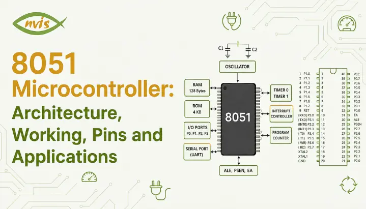
8051 Microcontroller: Architecture, Working, Pins and Applications

Posted on 27-08-202628-08-2026 by Tushar Saluja

TL;DR

This blog is for engineering freshers, university students, and GATE/SSC JE/RRB JE aspirants who want to understand 8051 microcontroller architecture from ground up, without getting lost in jargon.
8051 microcontroller packs a CPU, memory, timers, I/O ports, and a serial port onto a single chip, which is why it remains a commonly used teaching platform for learning embedded-system fundamentals in India.
This blog breaks down internal architecture, 40-pin layout, and how 8051 actually processes instructions, using plain language and a worked numerical example.
You will also see where 8051 fits into Indian engineering education, legacy industrial systems, automotive applications, and consumer electronics, along with its relevance to exams and embedded-systems careers.
By the end, you will be able to explain 8051 architecture confidently in interviews, labs, and competitive exams like GATE, SSC JE, and RRB JE.

The 8051 is an 8-bit microcontroller originally introduced by Intel in 1980. It uses a modified Harvard architecture, with separate program and data memory spaces. 8051-compatible devices are still offered by several semiconductor manufacturers. It integrates a CPU, RAM, ROM, I/O ports, timers, and a serial communication port on a single chip, which is what separates a microcontroller from a microprocessor. This guide explains 8051 microcontroller architecture section by section, walks through its 40-pin configuration, and connects each concept to real applications and exam preparation for Indian engineering students.

What Is 8051 Microcontroller, and Why Does It Matter?

Consider a remote control for ceiling fans. Fans automatically adjust speed by simply pressing a button. There is no separate processor chip, no separate memory chip and no separate circuit to sense when you press the button inside that remote. It all resides on a single chip. The chip is a microcontroller.

In essence, a microcontroller is a very small computer that fits into one silicon chip. It is composed of a processor that performs thinking, memory that stores instructions and data, and input-output pins to communicate with the outside world such as buttons, motors, and displays. A traditional microprocessor typically relies on external memory and peripheral components, whereas a microcontroller integrates a processor, memory, and peripherals on a single chip. A microcontroller has all that built-in, making it cheaper, smaller and easier to design with.

The 8051 became a popular teaching platform because its relatively simple architecture makes concepts such as registers, timers, interrupts, I/O, and memory organization easier to demonstrate. Many Indian engineering programmes continue to use the 8051 to introduce students to microcontroller fundamentals before moving to newer platforms such as STM32 and ESP32. If you can describe how the 8051 fetches, decodes, and executes an instruction, you will understand the basic instruction-execution concepts that apply across many processors and microcontrollers.

8051 Microcontroller Architecture: Big Picture

Think of a small office with one manager (CPU) with a personal notepad (registers), a filing cabinet (RAM) in which to keep the daily paperwork, a locked archive (ROM) in which to keep the instructions to be used for the rest of the manager’s life, and telephone lines (I/O ports and serial port) for communicating with the outside world. All of the manager’s responsibilities can be accomplished in that one office. The architecture of the 8051 microcontroller is precisely like that.

The heart of the 8051 microcontroller architecture is an 8-bit CPU, meaning that it works with 8 bits (1 byte) of data. The classic 8051 uses an 8-bit data path and a 16-bit address space for program and external data memory. Because the 8051 uses separate 16-bit address spaces for program memory and external data memory, each address space can theoretically cover up to 64 KB. The 8051 uses 16-bit addressing for its program and external data memory spaces, allowing each space to address up to 64 KB.

major building blocks of architecture of 8051 microcontroller are:

The CPU is the “brain” and retrieves instructions from memory, decodes their meaning and carries them out sequentially. The CPU contains Arithmetic Logic Unit (ALU) that carries out addition/subtraction and logical comparisons, accumulator (ACC) – a special register that stores the outcome of most operations.

memory is divided into two distinct memory spaces, program memory and data memory, This separation of program and data memory spaces is a defining characteristic of the 8051’s modified Harvard architecture. In contrast, a conventional Von Neumann architecture uses a shared memory space for instructions and data. In the original 8051, the on-chip program memory is 4 KB of ROM, while the internal RAM is 128 bytes. Program memory stores the program code, while RAM stores temporary data used during execution.

The chip can read switches, sensors, and buttons through four, 8-bit-wide I/O ports (P0, P1, P2, P3) and control LEDs, motors, and displays.

timers and counters, two of which are 16 bits, provide accurate time delays and counting of external events which are critical for many timing operations, such as flashing an LED at a specific time interval or counting the speed of a motor.

The 8051 has a full-duplex serial port that can transmit and receive data serially. Its TXD and RXD lines are available on P3.1 and P3.0 respectively, and the serial interface supports UART-style communication.

An interrupt system will allow the microcontroller to stop what it’s doing and react to some very urgent process, such as a button being pressed, without having to continuously scan for the event in a loop.

CPU: Decision-Making Core

Imagine a calculator that has a memory for the function just performed and that can determine what to do next based on the results of that function. It’s basically the 8051 CPU. It has ALU for arithmetic and logic operations, accumulator (register A), a special register named B that is used during multiply and divide operations, a group of general purpose registers (R0 to R7) used as temporary scratch pads.

CPU also has a special register called a Program Status Word (PSW) that contains bits that can be used as dashboard status lights. It contains status flags such as Carry (CY), Auxiliary Carry (AC), and Overflow (OV), along with register-bank selection bits and the parity flag. The classic 8051 PSW does not have a dedicated zero flag. These flags are continually scanned by a programmer to determine its value and thereby make a decision, just as you look at the fuel light in your car before you stop for petrol.

Memory Organization: Two Separate Filing Systems

This is a very practical analogy with which to work. Program memory is like a recipe book because it stores the instructions the CPU follows. Data memory is like a kitchen counter because it temporarily holds the data and values being worked on. The recipe book represents program memory because it stores the instructions the CPU follows, while the kitchen counter represents RAM, where temporary data can be read and changed during execution. Ingredients are placed on the kitchen counter and you can mix things and constantly update on what’s happening in the kitchen. With 8051, the ROM was like a recipe book, and the RAM was like a kitchen counter.

The original 8051 has 4 KB of on-chip program ROM and 128 bytes of internal RAM. It can also address up to 64 KB of external program memory and up to 64 KB of external data memory. Program ROM retains the stored program even when power is removed, which is why it is classified as non-volatile memory.

Data memory (RAM) is 128 bytes. The lower 32 bytes contain four register banks, the next 16 bytes are bit-addressable, and the remaining 80 bytes are general-purpose RAM. Special Function Registers (SFRs) are located in a separate address space from this 128-byte internal RAM.

The 8051 uses separate program and data memory spaces, allowing code and data to be addressed independently. This separation is a key characteristic of its modified Harvard architecture.

Worked Example: Suppose you want to know how many distinct memory locations 8051’s 16-bit address bus can access. A 16-bit address bus can represent 2^16 combinations, since each bit can be either 0 or 1.

2^16 = 65,536 locations, which equals 64 KB.

This is why you will often see “64 KB program memory” and “64 KB external data memory” mentioned in 8051 datasheets. 16-bit address bus is physical reason behind that 64 KB limit, and this exact kind of calculation shows up regularly in GATE and PSU written exams when they ask you to compute addressable memory from bus width.

Timers and Counters: Keeping Time Without a Wristwatch

Suppose you want the LED to turn on and off precisely once every second, without having to count seconds. There’s a component in the chip that can reliably count clock pulses, but your main program is doing other work, i.e. you want a clock to count in the background. That’s the job of Timer 0 and Timer 1.

Each timer uses a 16-bit counting register. In timer mode, it increments based on the internal machine-cycle timing; in counter mode, it increments in response to external transitions applied to its counter input, such as counting the number of times the conveyor belt sensor is triggered. When the timer is filled to its maximum value and wraps around to zero again, it may interrupt your program and indicate that a fixed period of time has elapsed.

The timers are configured and controlled using the 8-bit TMOD (Timer Mode) and TCON (Timer Control) registers. The timer modes determine whether the timer operates as a 13-bit timer, 16-bit timer/counter, 8-bit auto-reload timer, or, for Timer 0, two separate 8-bit timers.

I/O Ports: Chip’s Hands and Ears

The only real connection between 8051 and the physical world is the 8 pins per port (P0, P1, P2, P3) for a total of 32 general purpose I/O lines.

Port 0 is special as it serves double purpose. In designs that do not use external memory, Port 0 can be used as a general-purpose bidirectional I/O port, but it requires external pull-up resistors because it does not have internal pull-ups in the classic 8051. In larger designs, in which external memory is connected, Port 0 carries a lower byte of address and data, multiplexed onto the same pins; this is a smart use of pin space on the chip.

Most variants of the 8051 do not have an alternative function for port 1, making it the easiest port to use for simple input/output (I/O) applications, such as attaching LEDs and switches.

Port 2 can be used as general-purpose I/O or, when external memory is accessed, it carries the higher-order address byte (A8–A15).

The port 3 has multiple alternate functions that are vital to the operation of the chip, such as serial port’s transmit and receive lines, two external interrupt inputs, and the external count input for the timer.

Pin Diagram and Pin Description of 8051 Microcontroller

The 8051 microcontroller is packaged as a 40-pin Dual Inline Package (DIP), and understanding what every pin does is what actually lets you wire a circuit or answer a pin-diagram question correctly in an exam. Here is a pin-by-pin breakdown.

Pins 1 to 8 form Port 1 (P1.0 to P1.7), a general-purpose bidirectional I/O port with no alternate functions in base 8051, making it the simplest port to use for connecting external devices like LEDs or push buttons.

Pin 9 is RST, Reset pin. Applying a HIGH level to the RST pin for at least two machine cycles while the oscillator is running resets the microcontroller and places its registers and control logic into their defined reset states, similar to restarting your computer when it freezes.

Pins 10 to 17 form Port 3 (P3.0 to P3.7), which carries important alternate functions: P3.0 (RXD) and P3.1 (TXD) handle serial communication, P3.2 (INT0) and P3.3 (INT1) are external interrupt inputs, P3.4 (T0) and P3.5 (T1) are external timer/counter inputs, and P3.6 (WR) and P3.7 (RD) control write and read operations to external memory.

Pin 18 and Pin 19 (XTAL2 and XTAL1) connect to an external crystal oscillator, which generates clock pulses that drive every internal operation, similar to a heartbeat that keeps the whole chip synchronized.

Pin 20 is GND, ground reference for the entire chip.

Pins 21 to 28 form Port 2 (P2.0 to P2.7), used as general I/O, or as higher-order address byte (A8 to A15) when external memory is connected.

Pin 29 is PSEN (Program Store Enable), an output pin that goes active-low specifically when the CPU reads from external program memory.

Pin 30 is ALE (Address Latch Enable), used to separate multiplexed address and data signals on Port 0 during external memory access.

Pin 31 is EA (External Access), which decides whether CPU executes code from internal ROM or external memory. For the classic 8051, EA determines whether program execution uses the internal program ROM or external program memory. With EA high, the device uses its internal program memory for the internal address range; with EA low, it fetches program code from external memory

Pins 32 to 39 form Port 0 (P0.0 to P0.7), used as general I/O in small designs, or as multiplexed lower-order address and data bus (AD0 to AD7) in designs with external memory. Port 0 has no internal pull-up resistors, so external pull-ups are needed if you want to use it as a plain output port.

Pin 40 is VCC, supplying +5V power that runs the entire chip.

How 8051 Microcontroller Works: Instruction Execution Cycle

Think about how you follow a recipe. You read one line, understand what it is asking you to do, then actually do it, before moving to the next line. 8051 does exactly this with program instructions, in a loop called fetch-decode-execute cycle.

First, the CPU fetches an instruction from program memory (ROM), using Program Counter (PC), a register that always points to the address of the next instruction to be read. Second, the CPU decodes that instruction, figuring out what operation it represents, whether it is an addition, a data move, or a jump to another part of the program. Third, CPU executes instruction, actually performing operation, which might update the accumulator, change a flag in PSW, or toggle an I/O pin.

This entire cycle repeats continuously, driven by clock signals from external crystal oscillators connected at pins 18 and 19. The classic 8051 uses 12 oscillator periods per machine cycle. Therefore, with a 12 MHz oscillator, one machine cycle takes 1 μs, although individual instructions may require one or more machine cycles, though exact instruction execution time varies depending on how many machine cycles that particular instruction needs.

8051 vs 8052 vs 8031: Knowing Family

Students often get confused between these three names, so here is a plain difference. 8051 is the standard version with 4 KB of internal ROM and 128 bytes of RAM. 8052 is an upgraded version with double ROM (8 KB), double RAM (256 bytes), and an additional third timer, making it useful for slightly more demanding applications. 8031 is essentially an 8051-family device without on-chip program ROM, so it requires external program memory.

Feature	8051	8052	8031
Internal ROM	4 KB	8 KB	None (external only)
Internal RAM	128 bytes	256 bytes	128 bytes
Timers	2 (16-bit)	3 (16-bit)	2 (16-bit)
Interrupt sources	5	6	5
Typical use case	General teaching and small embedded designs	Slightly larger programs needing more memory	Designs already using external memory

Where 8051 Microcontroller Is Used in India

Even with modern 32-bit microcontrollers dominating new product designs, 8051 continues to have a real footprint in Indian industry and education, mainly because so much existing equipment, teaching infrastructure, and legacy code still runs on it.

Historically, 8051-based controllers have been used in simple industrial control applications such as relay control, instrumentation, and small automation systems. Today, newer microcontrollers are generally preferred for new industrial designs, while knowledge of 8051 can still be useful when working with legacy equipment and older control systems. Legacy 8051-based control boards can still be relevant when engineers maintain or troubleshoot older industrial equipment, although specific implementations vary by plant and system, and understanding this architecture helps engineers troubleshoot and maintain that equipment.

In consumer electronics, appliances like washing machines, microwave ovens, and remote controls historically ran on 8051 variants, and 8051-class devices can still be suitable for some simple, cost-sensitive embedded applications, although the specific microcontroller chosen depends on the product’s requirements and design constraints.

In automotive systems, 8051-family devices have been used historically in automotive and vehicle-related embedded applications, particularly in simpler control and instrumentation systems.Modern automotive designs generally rely on more capable automotive-grade microcontrollers and processors. ARM-based microcontrollers and software platforms such as AUTOSAR are widely used in modern automotive development, particularly as vehicle electronics become more complex.

In defense and aerospace, older microcontroller-based systems may use architectures such as the 8051, but newer systems generally use processors and microcontrollers selected according to their performance, reliability, radiation tolerance, and system requirements.

In engineering education, Many Indian engineering programs have historically used 8051 as an introductory platform for teaching microcontroller fundamentals, because its instruction set is simple enough to teach in a semester while still covering every core microcontroller concept students need before moving to ARM-based designs.

Exam Relevance: GATE, SSC JE, and RRB JE

If you are preparing for competitive exams, here is exactly where 8051 microcontroller fits into your syllabus. For GATE EC, the 2026 syllabus does not list 8051 as a dedicated topic. Students should therefore focus on broader concepts such as machine instructions, addressing modes, ALU, datapath and control unit, along with relevant embedded-systems fundamentals. Therefore, students should focus on the underlying concepts rather than treating 8051-specific memorization as a separate GATE syllabus area. The current GATE 2026 EC syllabus should be used as the reference when discussing exam relevance. Therefore, 8051-specific memorisation should not be treated as a separate GATE EC preparation area. Instead, focus on the broader computer-organisation and digital-electronics concepts covered by the official syllabus.

For SSC JE and RRB JE preparation, 8051-related concepts may be relevant depending on the applicable syllabus and recruitment notification. Students should check the latest official syllabus before treating 8051 as a guaranteed topic. Depending on the recruitment notification and syllabus, questions may cover topics such as microcontroller architecture, pin functions, timers, interrupts, and addressing modes. Expect questions asking you to identify pin functions, calculate timer overflow values, or explain differences between Harvard and Von Neumann architecture using 8051 as a reference example.

In technical recruitment exams and interviews for electronics and embedded-systems roles, questions on 8051 fundamentals may be useful for assessing concepts such as timers, interrupts, memory organisation, and I/O such as architecture, timers, interrupts, and memory organization, since these fundamentals demonstrate whether a candidate genuinely understands embedded systems or has only memorized definitions.

Career and Salary Relevance for Embedded Systems Roles in India

Learning 8051 architecture can provide a useful foundation in embedded-systems concepts, especially for students and beginners, even though most production work today happens on more advanced 32-bit microcontrollers.

Freshers entering embedded systems roles in India can see a wide range of starting compensation depending on location, company, skills, internships, and role requirements, with exact figures depending on internships, hands-on project experience, and whether the candidate has exposure to modern platforms alongside fundamentals like 8051. Candidates who pair 8051-level architectural understanding with practical skills on platforms like STM32, AVR, or ESP32 tend to command the higher end of that range, since companies want engineers who understand fundamentals but can also work on current hardware.

Mid-level embedded engineers with three to five years of experience in India typically earn higher salaries than freshers, with compensation varying significantly by experience, location, company, and technical specialization. Senior embedded engineers and architects at major semiconductor and automotive companies can earn substantially more. Demand driving this growth includes India’s semiconductor manufacturing push under PLI scheme, expanding EV sector, and growing IoT adoption across industrial and consumer products.

For freshers, practical takeaway is this: learning 8051 microcontroller architecture thoroughly builds conceptual foundation, including memory organization, interrupts, timers, and register-level programming, that transfers directly to every other microcontroller you will work with in your career, from AVR to ARM Cortex-M.

Conclusion

8051 microcontroller architecture might be decades old, but it remains a clear and useful way to understand how many fundamental microcontroller concepts work, from CPU and memory organization to timers, I/O ports, and the instruction-execution cycle used by processors and microcontrollers. You now know how its 40 pins are organized, how its Harvard architecture separates program and data memory, and where this chip still shows up in Indian industry, exams, and interviews today.

The best next step is hands-on practice. Pick up an 8051 development board, write a simple LED-blinking program using Timer 0, and watch concepts from this blog come alive on actual hardware. If you are preparing for SSC JE, RRB JE, or a PSU interview, revisit pin diagrams and timer sections until you can redraw and explain them without looking back at your notes.

FAQs

What is the 8051 microcontroller used for?

The 8051 microcontroller is used in embedded systems that need to control hardware directly, including industrial automation panels, consumer appliances, basic automotive dashboard controls, and countless college and hobbyist projects. Its simplicity makes it ideal for learning core microcontroller concepts before moving to advanced platforms.

What is the architecture of the 8051 microcontroller based on?

The architecture of the 8051 microcontroller is based on a modified Harvard architecture, meaning program memory and data memory occupy separate address spaces, which is a defining characteristic of the 8051’s modified Harvard architecture.

How many pins does an 8051 microcontroller have, and what are they used for?

The 8051 microcontroller has 40 pins in its standard DIP package. Of these, 32 pins form four 8-bit I/O ports (P0 to P3), while remaining 8 pins handle power supply, ground, reset, crystal oscillator connections, and control signals for external memory access.

Is 8051 microcontroller still relevant in 2026?

Yes, though mainly for education, legacy system maintenance, and cost-sensitive consumer products rather than new high-performance product design. Many new embedded projects use more capable 32-bit microcontrollers and SoCs, including STM32-family devices and ESP32-family chips, but 8051 architecture remains a commonly used teaching example for introducing microcontroller fundamentals because it clearly demonstrates core concepts every embedded engineer needs.

What is the difference between a microprocessor and an 8051 microcontroller?

A microprocessor, like ones in laptops, only contains CPU and needs external chips for RAM, ROM, and I/O. 8051 microcontroller integrates CPU, RAM, ROM, I/O ports, timers, and a serial port all on a single chip, making it self-sufficient for embedded applications without needing external support circuitry.

How many timers does an 8051 microcontroller have?

standard 8051 has two 16-bit timers, Timer 0 and Timer 1, used for generating precise time delays or counting external events. upgraded 8052 variant adds a third timer, useful for applications needing an additional independent timing source.

STM32 Microcontroller Guide: How It Works, Programming, and Applications

Posted on 27-08-202627-08-2026 by Tushar Saluja

TL;DR

This blog is for engineering students, freshers, and first-time embedded learners in India who want to learn about STM32 microcontrollers from scratch without prior experience in microcontroller programming.
STM32 is a range of 32 bit microcontroller chips from STMicroelectronics based on ARM Cortex M processor cores, and is one of the world’s most widely used 32bit microcontroller families.
This guide is designed to explain the STM32 uses and family of chips (STM32F, STM32L, STM32H, STM32G, STM32WB, STM32WL series), as well as how to program an STM32 using STM32CubeIDE, and finally has two worked numerical examples included for exam preparation.
It also elaborates on the context of India embedded technology based on STM32 used in the Indian industry, relevance of GATE & PSU exams and realistic salary expectations for embedded freshers.
At the end of this, you will be able to select a board, configure STM32CubeIDE and see what is now happening in the chip when the code is executed.

STM32 is a range of 32 bit microcontroller chips from STMicroelectronics based on ARM Cortex M processor cores. It is one of the most popular microcontroller platforms in use today in embedded systems applications ranging from the student robotics project to an industrial automation system or an automotive control unit. This guide explains the internal working of STM32 microcontroller, the difference between various series of STM32, how to program an STM32 using the STM32CubeIDE and the role of STM32 in engineering career and competitive exams in India.

What Is an STM32 Microcontroller?

Consider the differences between your laptop and a smart washing machine. Your laptop is a general purpose computer. It can run a browser, edit a video, play a game, and hundreds of other things, depending upon what software you install. There’s another computer in a washing machine, but it’s very small, and it does just one thing: runs the washing cycle, detects water level, controls the washing machine motor, and sounds a beep when it’s finished. Does not require a screen, keyboard or browser.

The microcontroller that’s in the washing machine is a small, single-purpose computer. One particular, very popular family of that dedicated computer is the STM32.

An STM32 microcontroller, technically speaking, is a 32 bit embedded computing chip that is based on an ARM Cortex M processor core. An STM32 integrates a processor core, Flash memory, SRAM, and a range of input/output peripherals on a single chip. The firmware required for the application is stored in the microcontroller’s non-volatile memory, typically Flash, and is executed when the device starts. You program the chip and store the program in its built-in flash memory, after which the STM32 executes the program whenever the device is powered on, continuing until power is removed or the microcontroller is reset.

This single chip design is a big reason why you see STM32 microcontrollers everywhere: from fitness bands and electric scooter controllers to industrial sensors and drone flight controllers used in student projects.

Why STM32 and Not Just Any Microcontroller?

If you’ve ever programmed with Arduino boards, you’ve already been working in microcontroller mode. Many classic Arduino boards, such as the Arduino Uno, use 8-bit AVR microcontrollers. It is relatively easy to learn and remains a good starting point for beginners. However it is slower, has less memory, and fewer built-in peripherals.

An STM32, on the other hand, is a 32 bit chip. To illustrate, consider two students working on the same math problem. The numbers can be worked with one at a time, with constant carry-over. Others can perform with significantly higher numbers in a single operation. A 32-bit STM32 can process 32-bit data types efficiently and generally offers more processing capability than many classic 8-bit microcontrollers. However, performance also depends on clock speed, instruction set, memory architecture, peripherals, and the specific MCU.

Unlike most beginner boards, STM32 has a much more extensive range of built-in peripherals. Multiple timers, multiple communication interfaces (UART, SPI, I2C, CAN, USB), high resolution analog to digital converters, and in many models, hardware security features. This is why engineers are choosing STM32 microcontrollers to go beyond a hobby project and onto production grade embedded systems and why the term stm32 microcontroller is frequently mentioned in embedded systems job announcements and project reports.

However, STM32 is not beyond the reach of the newbie. STMicroelectronics offers no cost graphical configuration tools, and the many problems which a new user of this system will face have already been solved by a large community.

Inside an STM32: How It Actually Works

Open up an STM32 chip conceptually, and you will find four main building blocks working together. Understanding these four pieces is the real foundation of learning any stm32 microcontroller, because every tutorial, every CubeIDE setting, and every line of code eventually ties back to one of them.

Processor Core: Brain That Follows Instructions

At the center sits ARM Cortex M core. Picture a diligent assembly line worker who fetches one instruction at a time from program memory and executes exactly what it says: add these two numbers, check this condition, turn on this pin. That is what the processor core does, millions of times per second.

STM32 uses different variants of this Cortex M core depending on the series. Cortex M0 and M0+ are simplest and most power efficient, good for basic tasks like blinking LEDs or reading a single sensor. Cortex M3 offers a balanced middle ground. Cortex M4 adds digital signal processing and floating point math support, useful for motor control or audio work. Cortex M7 is a powerhouse, built for heaviest computational loads like real time image processing.

core also manages interrupts through a component called NVIC, or Nested Vectored Interrupt Controller. Think of an interrupt as a phone call that arrives while you are doing homework. You pause what you are doing, answer calls, then return to homework exactly where you left off. That is precisely how an STM32 handles a button press or an incoming data byte while running its main program loop.

Memory: Where Program and Data Live

Every STM32 has two main types of memory. Flash memory is like a notebook with permanent ink. Your compiled program is written here, and it stays even after power is switched off. SRAM stores temporary data such as variables, stack contents, and buffers while the program runs. Its contents are not retained when power is removed.

A typical entry level STM32F103 chip, for example, offers 64 KB of flash memory and 20 KB of SRAM. That sounds tiny compared to a laptop’s gigabytes, but for a dedicated task like reading a temperature sensor and controlling a fan, it is more than enough.

GPIO Pins: How Chip Talks to Outside World

GPIO stands for General Purpose Input Output, and these are physical legs of the chip that connect it to LEDs, buttons, motors, and sensors. STM32 groups these pins into ports labeled PA, PB, PC, and so on, with individual pins named PA0, PA1, PB5, and similar.

Each GPIO pin is flexible. It can be configured as a digital input to read a button press, a digital output to switch an LED, an analog input to measure a varying voltage, or an alternate function pin that hands control over to a built-in peripheral like UART or SPI. This flexibility is configured through the microcontroller’s software and peripheral configuration tools such as STM32CubeMX.

Clock System and Peripherals: Heartbeat and Toolkit

Every STM32 needs a clock signal, essentially a heartbeat that ticks at a fixed rate and tells every part of the chip when to move to the next step. STM32 chips can generate this clock internally or use an external crystal, and a Phase Locked Loop, or PLL, can multiply that base frequency up to chip’s maximum speed when more performance is needed.

Around this clock, STM32 wraps a rich set of peripherals, small specialized circuits that handle specific jobs so the main processor does not have to. Timers measure time intervals and generate PWM signals for motor speed control. An ADC, or Analog-to-Digital Converter, converts a real-world analog voltage, such as the output of a temperature sensor, into a digital value that the processor can use. UART, SPI, and I2C handle serial communication with other chips and modules. DMA, or Direct Memory Access, moves data between memory and peripherals without tying up the processor at all.

STM32 Family: Which Series Does What

STMicroelectronics does not make just one STM32 chip. It makes dozens, grouped into series, each tuned for a different job. Picking the right one is a lot like picking the right vehicle: a delivery scooter, a family sedan, and a cargo truck are all vehicles, but you would not use them interchangeably.

Series	Cortex M Core	Best For	Typical Use Case
STM32F0 / F1	M0 / M3	Learning, general purpose control	Student projects, Blue Pill boards
STM32F4	M4	Performance with DSP and floating point	Motor control, audio, robotics
STM32H7	M7	Maximum computational power	Industrial automation, signal processing
STM32L	M0+ / M4	Ultra low power	Battery powered IoT, wearables
STM32G	M0+ / M4	Balanced performance and efficiency	Modern sensing and control systems
STM32WB / WL	M4	Wireless connectivity built in	Bluetooth LE and other wireless connectivity

STM32F1 series, home to the famous STM32F103C8T6 chip found on Blue Pill boards, is where most Indian students take their first step into STM32, largely because it is inexpensive and well documented. Once a learner is comfortable, moving to an STM32F4 for a robotics or drone project, or an STM32L series chip for a battery powered IoT device, becomes a natural next step.

Getting Started: STM32CubeIDE and Your First Program

Good news for beginners is that STMicroelectronics provides STM32CubeIDE as a free development environment for editing, compiling, programming, and debugging STM32 projects. STM32CubeMX is available separately for graphical device configuration and code generation is now available as a separate graphical configuration and initialization-code generation tool within the STM32Cube ecosystem. You do not need to buy Keil or IAR licenses to get started, though professional teams sometimes use those tools too.

Here is what the first time workflow looks like, step by step.

Step 1: Install STM32CubeIDE. Download it free from the official ST website and install it like any other application.

Step 2: Create a new project and select your chip. Select your STM32 device or board according to the development workflow you are using. STM32CubeMX can be used to configure the device, pins, clocks, and peripherals and generate the project files, which you can then build and debug using STM32CubeIDE.

Step 3: Configure your pins visually. Instead of writing low-level register configuration by hand, you can use STM32CubeMX to select pins and configure functions such as GPIO, ADC, UART, SPI, and other peripherals through a graphical interface, output, input, ADC, or a peripheral like UART. This step alone removes most of the intimidation factor that used to make microcontroller programming difficult for beginners.

Step 4: Set clock configuration. STM32CubeMX provides a graphical clock configuration view where you can configure the system clock and peripheral clock settings.

Step 5: Generate initialization code. STM32CubeMX can generate the low-level initialization code based on your pin, clock, and peripheral configuration. You can then open or import the generated project into your chosen development environment, such as STM32CubeIDE.

Step 6: Write your application logic. This is where you add your own code, typically inside a while(1) loop that runs forever. A classic first program toggles a GPIO pin connected to an LED, using HAL_GPIO_TogglePin() function along with HAL_Delay() to add a pause, creating a well known blinking LED result.

Step 7: Connect your ST Link programmer and flash code. Most STM32 development boards, including Nucleo series, have a built in ST Link programmer, so a single USB cable is all you need. Click the run button, and your compiled program is written directly into the chip’s flash memory.

Step 8: Debug if needed. STM32CubeIDE includes a built in debugger, letting you pause your program mid execution and inspect variable values in real time, which is invaluable when a sensor reading looks wrong and you need to find out why.

Worked Numerical Examples

Numerical problems on microcontrollers show up often in university lab exams and in GATE style objective questions. Here are two worked examples that reflect the kind of calculation you are likely to face.

Example 1: ADC Voltage Calculation

An STM32’s ADC is 12 bit, meaning it converts an analog voltage into a digital value between 0 and 4095. Suppose ADC reference voltage is 3.3 V, and a temperature sensor produces a raw ADC reading of 2048. What is the actual input voltage?

formula is:

Voltage = (ADC reading / Maximum ADC value) × Reference voltage

Voltage = (2048 / 4095) × 3.3 V

Voltage = 0.5001 × 3.3 V

Voltage ≈ 1.65 V

This makes sense intuitively too: 2048 is almost exactly half of 4095, so the result should land close to half of 3.3 V, which it does.

Example 2: PWM Frequency Calculation

STM32 timers generate PWM signals using two settings: Prescaler (PSC) and Auto Reload Register (ARR). Suppose the timer’s input clock is 72 MHz, prescaler is set to 71, and ARR is set to 999. What PWM frequency does this produce?

First, find timer’s counting frequency after prescaler divides it down:

Counting Frequency = Timer Clock / (PSC + 1)

Counting Frequency = 72,000,000 / (71 + 1) = 72,000,000 / 72 = 1,000,000 Hz (1 MHz)

Next, find PWM output frequency using ARR:

PWM Frequency = Counting Frequency / (ARR + 1)

PWM Frequency = 1,000,000 / (999 + 1) = 1,000,000 / 1000 = 1000 Hz

So this timer configuration produces a 1 kHz PWM signal, a common setting for controlling speed of a small DC motor or brightness of an LED.

STM32 in India: Boards, Pricing, and Where It’s Used

Cost is an important consideration for students, and low-cost STM32 development boards are widely available in India. The STM32F103C8T6 Blue Pill is a low-cost STM32 development board commonly used by students and hobbyists which is available in the market at a low price at various platforms such as Robu.in, Robocraze, Flipkart, etc., and provides an inexpensive way to experiment with an STM32F103C8T6 32-bit ARM Cortex-M3 microcontroller. Official STM32 Nucleo boards are shield compatible with Arduino, include a built-in STM32 programmer and are more expensive.

STM32 is used not only in student and hobby projects but also across several industrial applications in India. STM32 microcontrollers can be used in automotive, EV, industrial automation, consumer electronics, and IoT applications. India’s growth in EVs and electronics manufacturing is also increasing demand for embedded-system skills, although the use of a specific MCU family varies by company and product for EVs. STM32 devices are suitable for industrial automation applications such as controllers, monitoring systems, and human-machine interfaces (HMIs), although the specific MCU used varies by product and company. India’s growth in electronics manufacturing and government initiatives supporting electronics production are contributing to broader opportunities in embedded hardware and firmware. However, the impact varies by company and product.

STM32-based embedded development is not limited to one sector. Microcontrollers are used across industrial automation, automotive, consumer electronics, IoT, power systems, and other embedded applications, although the specific MCU family depends on the product and its requirements. However, the specific MCU families used by individual organizations and projects vary, so STM32 should not be presented as the standard platform across these organizations without a specific source. Organizations such as BEL and companies in the power sector use automation, monitoring, control, and embedded technologies. However, the specific microcontroller families used in their projects vary by system and application.

GATE, ISRO, DRDO and Exam Relevance

Microcontroller, digital electronics, computer organization, and embedded-system concepts are relevant to several engineering examinations and technical recruitment processes in India, and STM32 is practical, hands on face of concepts that otherwise stay purely theoretical.

For ECE students, GATE covers related areas such as digital circuits, data converters, semiconductor memories, and computer organization. These topics overlap with several STM32 fundamentals, although GATE does not require students to study the STM32 platform specifically. For ECE and EE students, this means questions on interrupts, timers, memory mapped I/O, and ADC principles, all of which map directly onto what you configure inside STM32CubeMX.

Some DRDO recruitment routes use GATE scores as part of the selection process, while requirements vary by post and recruitment notification. ISRO also uses recruitment processes that vary by post and recruitment cycle. Candidates should always follow the latest official notification and syllabus, including written tests and/or GATE-based shortlisting depending on the notification. ISRO recruitment uses its own selection process and technical assessment, so candidates should prepare according to the current recruitment notification and syllabus rather than assuming that it follows GATE’s pattern. Practical STM32 project experience can also help demonstrate hands-on embedded-system skills during technical interviews, although selection criteria vary by organisation and recruitment cycle.

For SSC JE and RRB JE aspirants, relevant electronics and digital-system fundamentals may overlap with topics such as digital electronics, basic circuits, and instrumentation, but candidates should follow the syllabus for their specific examination. Even if the exam itself does not name STM32 directly, understanding how a real microcontroller handles GPIO, interrupts, and communication protocols makes underlying digital electronics theory click far faster than memorization alone.

Career and Salary Guide for STM32/Embedded Freshers

STM32 experience is one of more direct paths from a college project to a paying embedded systems role in India, STM32 is a useful skill for embedded-systems candidates because job postings often mention it alongside ARM Cortex-M, C/C++, RTOS, and communication protocols.

For freshers with zero to two years of experience, embedded systems salaries in India typically range from roughly 3 to 6 LPA, though Strong STM32 projects can strengthen a fresher’s portfolio, particularly when they demonstrate practical skills such as peripheral configuration, communication protocols, debugging, and sensor interfacing. Some listings for embedded software and system engineer roles requiring STM32 alongside RTOS and Linux experience post significantly higher ranges, though these typically expect a few years of prior experience rather than being fresher friendly.

Job postings for embedded roles often list STM32 alongside skills such as C/C++, RTOS, ARM Cortex-M, and communication protocols such as UART, SPI, and I2C. Postings frequently ask for STM32 alongside ESP32 and other platforms like Nordic nRF and Silicon Labs, plus serial communication protocol experience, and roles often expect working knowledge of ARM Cortex based microcontrollers interfaced with memory, RTC, and sensors over SPI, UART, and I2C. This tells you the practical shape of a strong fresher resume: an STM32 project that actually talks to a sensor over I2C or SPI, sends data out over UART, and ideally saves data to some form of memory, generally demonstrates more practical ability than a basic blinking-LED demonstration.

Bengaluru, Pune, Hyderabad, Chennai, and other major technology and automotive hubs have significant embedded-systems activity, spanning industrial automation, automotive, and defence electronics employers. As experience grows, so does pay band, with mid level embedded engineers moving well past fresher range as they take on RTOS, driver level, and system architecture responsibilities.

Conclusion

An STM32 microcontroller is best understood not as an intimidating chip full of registers, but as a small, dedicated computer built to do one job reliably, using an ARM Cortex M core, on chip memory, GPIO pins, and a set of hardware peripherals that all work together. Once that mental model is in place, Tools such as STM32CubeMX can simplify initial device, pin, clock, and peripheral configuration through a graphical interface, while STM32CubeIDE provides the environment for developing, compiling, programming, and debugging the application.

For Indian students, the path forward is clear and inexpensive: pick up an STM32F103 Blue Pill or a Nucleo board, walk through blinking LED examples, then build one project that actually reads a sensor and talks to it over UART, SPI, or I2C. That project can reinforce practical concepts related to microcontrollers, digital systems, communication interfaces, and embedded programming, while also strengthening your embedded-systems resume while also becoming the centerpiece of your first embedded systems resume. Start with hardware you can afford today, and let projects grow from there.

FAQs

Is STM32 good for beginners with no prior microcontroller experience?

Yes. While STM32 has a steeper learning curve than Arduino, tools like STM32CubeIDE and STM32CubeMX handle most of low level setup visually, so a beginner can get a working project running without writing register level code. Starting with an inexpensive STM32F103 board and following a structured tutorial is a realistic first step for any engineering student.

What is the difference between STM32 and Arduino?

Arduino refers to a development board and ecosystem, some of which use STM32 chips internally, while STM32 refers specifically to STMicroelectronics’ family of 32 bit ARM Cortex M microcontroller chips. STM32 generally offers more processing power, more memory, and more built in peripherals than 8 bit AVR chips used in classic Arduino boards, making it better suited for advanced or performance heavy projects.

Do I need to know C programming before learning STM32?

Yes, a working knowledge of C is expected, since STM32 firmware is written almost entirely in C or C++. You do not need to be an expert, but you should be comfortable with variables, functions, pointers, and basic data types before starting STM32 development.

Which STM32 board should a first time student in India buy?

STM32F103C8T6 Blue Pill is the most common and affordable starting point for Indian students, widely available through Robu.in, Robocraze, and similar platforms. Students who want a built-in. programmer and easier debugging often prefer an official STM32 Nucleo board instead, at a somewhat higher price.

Does STM32 knowledge help with GATE or PSU exams like ISRO and DRDO?

STM32 itself is generally not tested as a specific platform. However, working with STM32 can help students understand practical concepts such as GPIO, timers, interrupts, ADCs, memory, and communication interfaces. These concepts can complement preparation for relevant electronics and computer-organization topics.

What is STM32CubeIDE used for?

STM32CubeIDE is STMicroelectronics’ free development environment for STM32 microcontrollers. It provides tools for editing, compiling, programming, and debugging STM32 projects. STM32CubeMX is available separately for graphical pin, clock, and peripheral configuration and code generation, covering the entire STM32 development workflow in a single free download.

Ward Leonard Method of Speed Control: Working Principle, Advantages and Disadvantages

Posted on 20-08-202620-08-2026 by Tushar Saluja

TL;DR

This blog is for electrical engineering students, GATE and SSC JE aspirants, and freshers who want to understand Ward Leonard method of speed control with a clear, exam ready explanation rather than a dry textbook definition.
Ward Leonard system controls a DC motor’s speed by changing voltage fed to it, using a separate motor generator set instead of resistors or switches.
It became one of the smoothest and widest-range speed-control methods for DC motors and was widely used for decades in elevators, steel mills, mine hoists, cranes, and other demanding industrial applications.
A worked numerical example, comparison table, and India specific industrial context are included to help you connect theory to real plants and real exam questions.
Modern power-electronic drives, including thyristor DC drives and, where AC motors are used, VFDs, have largely replaced Ward Leonard systems.

Imagine trying to slow down a car by dragging your foot on the road instead of easing off the accelerator. It would work, technically, but you would waste a lot of energy as heat and wear out your shoe fast. Early speed control methods for DC motors had a similar problem. Engineers controlled speed by inserting resistors into the circuit, which wasted power as heat, gave a limited speed range, and could not push the motor above its normal speed smoothly.

Ward Leonard method of speed control solved this problem by changing strategy entirely. Instead of wasting energy through resistors, it changes voltage supplied to the motor directly, using a dedicated generator built just for that purpose. This single idea, controlling speed through variable voltage rather than variable resistance, became one of most important developments in the history of electric drives.

This blog breaks down Leonard’s system of speed control the way a mentor would explain it on a whiteboard: starting from everyday logic, moving into technical working, and ending with exact things you need for your GATE, SSC JE, or RRB JE preparation.

What Is the Ward Leonard Method of Speed Control?

Picture two water tanks connected by a pipe. If you want more water to flow through the pipe, you do not squeeze the pipe narrower and force water through it. You simply raise the water level in the first tank, and flow increases naturally with more pressure. Ward Leonard method applies exactly this logic to electricity.

In a DC motor, speed depends almost directly on voltage applied to its armature. Higher voltage means higher speed, and lower voltage means lower speed, as long as field current stays constant. So instead of restricting current with resistors, Ward Leonard method varies voltage itself, smoothly and continuously, using a generator whose output can be adjusted at will.

The Ward Leonard method of speed control was introduced by American engineer Harry Ward Leonard in 1891. His idea was simple but powerful. Take a constant speed AC or DC motor, couple it mechanically to a separately excited DC generator, and let that generator supply variable DC voltage to the motor you actually want to control. Change generator’s field current, and its output voltage changes. Change output voltage, and the controlled motor’s speed changes right along with it.

This is why the Ward Leonard control system is often called an armature voltage control method. The field of the controlled motor remains untouched. For speeds up to the base speed, the Ward Leonard system controls the motor through variable armature voltage while keeping the motor field approximately constant. For speeds above the base speed, motor field weakening can be combined with armature voltage control to achieve a wider speed range.

Three Machines Behind Ward Leonard System

To really understand how this system works, it helps to think of it as a small team of three machines, each with one job.

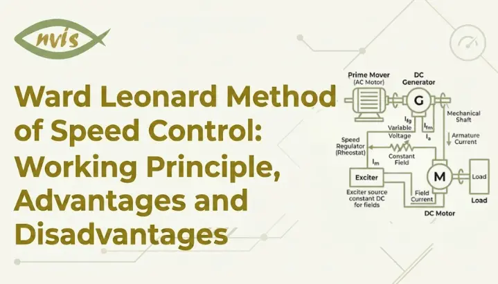
A driving motor is a constant speed machine that keeps everything running. It is usually a three phase induction motor or a synchronous motor, connected directly to the main AC supply, and it always spins at a fixed speed. Its only job is to provide mechanical power to turn the generator.

The generator is coupled mechanically to the driving motor, so it always spins at that same constant speed too. But its electrical output is not fixed. By adjusting the generator’s own field current through a small rheostat, its output voltage can be raised or lowered smoothly from zero to its rated value, and even reversed in polarity.

A controlled motor, sometimes labelled M1 in textbook diagrams, is an actual DC motor whose speed you want to control. It receives its armature supply directly from the generator, while its field winding is separately excited and kept constant. Since motor speed depends on armature voltage, and generator’s voltage is fully adjustable, the controlled motor’s speed becomes fully adjustable too.

The combination of the driving motor and generator is called the motor-generator (MG) set. Together with the controlled DC motor, it forms the basic Ward Leonard system.

How Speed Control Actually Happens

Here is where the system becomes genuinely elegant. A field regulator, a small rheostat connected to the generator’s field winding, is the only control operator needs to touch.

When the generator’s field current is zero, its output voltage is zero, and the controlled motor stays still. As the operator gradually increases field current using rheostat, the generator’s output voltage rises smoothly from zero. This voltage is applied directly to the controlled motor’s armature, so the motor starts rotating and speeds up in proportion to rising voltage.

Because the generator voltage can be increased gradually from zero, the motor can start smoothly while its armature current remains within the required limit. Therefore, a separate conventional starting resistor is not normally required in the Ward Leonard arrangement.

Reversing direction is just as elegant. By reversing the generator’s field current using a simple reversing switch, the polarity of the generator’s output voltage flips. This reverses current through the controlled motor’s armature, which reverses its direction of rotation, all while the motor generator set keeps spinning in the same direction throughout.

There is one more capability that made this system genuinely ahead of its time. During regenerative braking, the generator output voltage is reduced below the motor’s induced back EMF. The motor then operates as a generator and sends electrical power back through the Ward Leonard set. The generator operates in the opposite energy-conversion direction, ultimately allowing the prime mover to return energy to the AC supply. The Ward Leonard system has inherent regenerative braking capability, although the control arrangement must be designed to provide the required operating conditions.

Worked Numerical Example

Numbers make this concept concrete, and this is exactly the kind of question that shows up in GATE and SSC JE papers.

Suppose a separately excited DC generator in a Ward Leonard system is driven at a constant speed and generates 220 V when its field current is at rated value. This voltage is applied directly to armature of a separately excited DC motor whose armature resistance is 0.5 ohm and whose back EMF constant relates speed and flux such that at 220 V armature voltage and rated flux, motor runs at 1000 RPM while drawing a full load armature current of 20 A.

If the generator’s field current is reduced so that its output voltage drops to 110 V, and motor’s field flux is kept unchanged, new operating speed can be estimated using the relationship that speed is proportional to armature voltage minus armature resistance drop, divided by flux.

At 220 V: back EMF equals 220 minus (20 times 0.5), which is 220 minus 10, giving 210 V, corresponding to 1000 RPM.

At 110 V, assuming the motor continues to drive a constant-torque load, the armature current remains approximately 20 A for simplicity. Therefore, back
EMF = 110 − (20 × 0.5) = 100 V.

Since speed is proportional to back EMF when flux is constant, new speed works out to 1000 multiplied by (100 divided by 210), which is approximately 476 RPM.

This shows core exam skill directly: halving generator’s output voltage very nearly halves motor’s speed, since armature resistance drop is small compared to applied voltage. This proportional relationship between generator field current, generator voltage, and motor speed is exactly what most GATE and SSC JE numericals on Ward Leonard method are testing.

Ward Leonard Ilgner System

Large industrial loads rarely stay constant. A steel rolling mill or a mine hoist can demand a sudden, massive surge of power for a few seconds and then fall quiet again. Feeding these spikes directly from the AC supply would cause the whole plant’s voltage to sag and flicker, disturbing every other machine connected to the same supply.

Ward Leonard Ilgner system solves this by adding a flywheel and a slip ring induction motor to standard setup. During normal, light load periods, induction motor spins flywheel up to speed, storing rotational energy in it. The moment a sudden heavy load hits a controlled motor, that stored rotational energy gets released, so the flywheel momentarily slows down while it takes on part of the load itself, easing the burden on incoming supply. Once demand eases off again, the induction motor quietly spins the flywheel back up, ready for the next surge.

This arrangement reduces the peak power drawn from the AC supply by allowing the flywheel to supply part of the sudden overload. As a result, the required power rating of the supply-side equipment and driving motor can be reduced compared with a system designed to handle the entire peak load directly. This is precisely why the Ilgner variant found its home in heaviest industrial applications, including blooming mill drives and colliery winders, where individual drive units can run into megawatt range.

Advantages of Ward Leonard System

The reason this system dominated precision drives for nearly a century comes down to a genuinely strong list of benefits.

With appropriate armature-voltage control and motor field weakening, the Ward Leonard system can provide a wide speed range; traditional references commonly quote a maximum-to-minimum speed ratio of about 20:1 to 40:1, depending on the design and control arrangement.

Starting is gentle by nature, since the generator’s output voltage rises from zero, which means the controlled motor accelerates smoothly and no separate starter is required at all.

Speed regulation under load is excellent, meaning the motor holds its set speed closely even as mechanical load on it changes.

Regenerative braking is an inherent capability of the Ward Leonard system. When the motor is driven above the speed corresponding to the applied armature voltage, it can operate as a generator and return electrical energy through the drive system to the supply, provided the control arrangement supports regenerative operation.

Because of all this, the system was, and in some legacy installations still is, a natural choice for jobs demanding frequent starting, stopping, and direction reversal, such as elevators, rolling mills, and excavators.

Disadvantages of Ward Leonard System

None of these benefits came free, and drawbacks are exactly why modern plants have largely moved away from this method.

The system needs three full electrical machines instead of one, driving motor, generator, and controlled motor, which makes initial cost very high.

All that extra machinery also means a much larger physical footprint, heavier installation, a costlier foundation, and significantly more floor space than a compact modern drive would need.

Overall efficiency suffers because power is converted twice, first from AC to mechanical to DC in the generator, and then from DC to mechanical again in the controlled motor, and this inefficiency gets worse when the system runs under light load.

Three rotating machines mean more maintenance requirements, more noise during operation, and more potential points of mechanical or electrical failure.

These downsides are precisely why solid state alternatives eventually took over, a shift covered in detail in the next section.

Applications of Ward Leonard Method

Despite its bulk and cost, Ward Leonard system found a home wherever precision mattered more than efficiency or space.

Elevators relied on this system for decades, since it offered smooth speed control and consistent torque, until thyristor drives became widely available in the 1980s.

Steel rolling mills used it to drive rollers that shape red hot steel, where even slight speed inconsistency can ruin an entire batch of material.

Mine hoists and colliery winders depended on it for safely raising and lowering personnel and material through deep shafts, where smooth acceleration and reliable braking are safety critical.

Paper mills used it to keep multiple stages of the manufacturing process running at precisely synchronised speeds, since a mismatch anywhere along the line damages paper.

Beyond heavy industry, Ward Leonard-type motor-generator systems were also used in applications requiring precise electromechanical positioning, where extremely smooth, precise motion it offered was exactly what gun directing systems needed.

Ward Leonard System vs Modern DC and AC Drives

Comparing the classic Ward Leonard method against drives that eventually replaced it makes trade offs much clearer.

Parameter	Ward Leonard System	Modern VFD / Thyristor Drive
Number of machines needed	Three (driving motor, generator, controlled motor)	One (motor itself, plus a compact electronic converter)
Physical size and weight	Very large, heavy, needs significant floor space	Compact, panel mounted, minimal footprint
Initial cost	High, due to extra rotating machines	Lower, though power electronics add their own cost
Efficiency	Reduced by double energy conversion, worse at light load	High, since power electronic conversion has fewer losses
Maintenance	Frequent, due to brushes, bearings, and commutators on three machines	Minimal, mostly solid state with far fewer moving parts
Noise	Noticeable, from rotating machinery	Very low
Response speed	Smooth but mechanically limited	Extremely fast, controlled electronically
Typical modern use	Legacy installations, some heavy industrial retrofits	Standard choice in nearly all new industrial drives

Is the Ward Leonard Method Still Used in India Today?

Walk through a modern Indian steel plant today and you will rarely find a classic Ward Leonard motor generator set still running main rolling stands. Modern Indian steel plants increasingly rely on PLC-based automation and modern power-electronic drives, including DC drives and VFDs, for rolling-mill and other variable-speed applications, which deliver same precise, wide range speed control Ward Leonard system once provided, but from a fraction of footprint and with far less maintenance overhead.

This does not make the Ward Leonard method irrelevant. It remains genuinely important for three reasons. First, some older Indian mills, mine hoists, and elevator installations still run on legacy Ward Leonard equipment, and engineers maintaining these systems need to understand exactly how they work. Second, the Ward Leonard system is an important historical foundation for modern variable-speed drive technology, particularly electronic DC drives. Modern VFDs use a different approach based on power-electronic conversion and frequency control of AC motors. Third, and most practically for students, this topic is a recurring favourite in GATE, SSC JE, and RRB JE electrical engineering papers, which means skipping it is not really an option if you are preparing for these exams.

Understanding the Ward Leonard system, in other words, is less about maintaining old machines and more about understanding the DNA of every drive system that came after it.

Career Relevance of Ward Leonard Speed Control

Electrical drives and motor control are not just exam topics. They translate directly into real, well paying career paths in India, and understanding classical systems like Ward Leonard gives you a genuine head start when you move on to studying VFDs, servo drives, and industrial automation.

Career Relevance for Electrical Engineers

Understanding DC drives, motor control, regenerative braking, and industrial automation can help electrical engineering students build a foundation for careers in electrical drives, industrial automation, power electronics, and maintenance engineering.

Specialising further pays off significantly. Engineers who build expertise in industrial automation, PLCs, SCADA systems, or power electronics can access specialised career opportunities because these skills are widely used in modern industrial and electrical systems. Since the Ward Leonard method is an important milestone in the development of variable-speed electrical drives, a solid grasp of it makes concepts like VFD tuning, regenerative braking in EVs, and closed loop motor control noticeably easier to pick up later.

For students still deciding where to specialise, drives and automation remain one of more resilient tracks in Indian electrical engineering, since virtually every steel plant, cement plant, paper mill, elevator manufacturer, and EV company needs engineers who genuinely understand how motor speed control works, not just how to operate a VFD panel by trial and error.

GATE, SSC JE, and RRB JE Exam Relevance

Leonard method of speed control shows up consistently across Indian electrical engineering competitive exams, and it is worth knowing exactly what form these questions usually take.

Conceptual questions typically test whether you understand that this is fundamentally an armature voltage control method, applicable to DC shunt and separately excited motors, and that it is not used for series or universal motors. Expect direct statements to verify as true or false, along with questions asking you to identify which machine’s field current is actually being varied to control speed, since students often confuse generator’s field with motor’s field.

Numerical questions, similar to worked examples earlier in this blog, usually give you a generator voltage, an armature resistance, a load current, and a known speed at one voltage, then ask you to calculate the resulting speed at a different generator voltage. A key relationship to remember is that back EMF is proportional to speed when flux is constant, and back EMF equals applied voltage minus armature current times armature resistance.

Application based questions test whether you know why this method suits loads requiring frequent starting, stopping, and reversal, and why it offers inherent regenerative braking without any additional circuitry, a point that is very commonly tested precisely because it distinguishes Ward Leonard from simpler resistance based control methods.

Comparison questions often ask you to contrast Ward Leonard with other DC motor speed control methods, namely armature resistance control and field flux control, focusing on efficiency, cost, and speed range as key differentiators.

Conclusion

Ward Leonard method of speed control took a simple, honest idea, that motor speed follows armature voltage, and built an entire mechanical electrical system around delivering that voltage smoothly and reliably. It gave engineers a highly effective wide-range, bidirectional speed-control system for DC motors, decades before modern power electronics could perform similar functions in a much smaller package.

To summarise key points from this blog: system uses three machines working together, a driving motor, a generator, and a controlled motor, with speed adjusted purely through generator’s field current. It excels at smooth, wide-range, bidirectional control and inherent regenerative braking capability when operated in regenerative mode, but pays for this with high cost, large size, and lower efficiency compared to modern drives. Ilgner variant added a flywheel to handle heavy intermittent industrial loads without disturbing the main power supply. And while VFDs and thyristor drives have replaced it in nearly all new Indian installations, the underlying principle remains foundational to every modern variable speed drive in use today.

If you are preparing for GATE, SSC JE, or RRB JE, make sure you can explain the working principle in your own words, solve a voltage to speed numerically confidently, and list advantages and disadvantages without hesitation. That combination covers almost everything examiners ask about this topic.

FAQs

What is the Ward Leonard method of speed control used for?

Leonard method of speed control is used to smoothly control speed of a DC motor, in both directions of rotation, across a very wide range. It was historically used in elevators, steel rolling mills, mine hoists, cranes, and paper mills, wherever precise, sensitive speed control mattered more than cost or size.

Who invented the Ward Leonard control system?

The system was introduced by American electrical engineer Harry Ward Leonard in 1891, and it went on to become one of most influential drive control methods of the twentieth century.

Is the Ward Leonard method still used in India?

Rarely for new installations. Most Indian steel plants and industries have shifted to VFDs and thyristor based drives, which offer similar precise control from a much smaller footprint. However, some legacy elevators, mine hoists, and older mill drives still run on Ward Leonard systems, and underlying principle remains foundational to how modern drives work.

What is the difference between the Ward Leonard system and Ward Leonard Ilgner system?

The standard Leonard control system uses a motor generator set alone. Ilgner variant adds a flywheel and typically a slip ring induction motor, allowing the flywheel to absorb sudden heavy load demands and release stored energy back into the system, which smooths out supply current fluctuations in large industrial drives.

What are the main disadvantages of the Ward Leonard method of speed control?

The biggest drawbacks are high initial cost from needing three separate machines, large physical size and floor space requirements, reduced efficiency due to double energy conversion, and higher maintenance needs compared to modern solid state drives.

Does the Ward Leonard method work for DC series motors?

No. This is a common exam trap. Leonard system of speed control is designed for DC shunt motors and separately excited DC motors, where field can be held constant while armature voltage is varied. It is not a standard method used for series motors.

Why is the Ward Leonard method important for GATE and SSC JE preparation?

It is a recurring topic in DC machines and electrical drives sections of these exams, tested through conceptual questions, numericals relating voltage to speed, and comparison questions against other speed control methods. Understanding it thoroughly also builds foundation for later topics like VFDs and closed loop motor control.

What Is a Ballistic Galvanometer? Working Principle, Formula & Experiments

Posted on 07-07-202608-07-2026 by Tushar Saluja

TL;DR

This blog is for engineering and physics students, especially university freshers preparing for electromagnetism labs, who want a clear, beginner friendly explanation of what a ballistic galvanometer is and how it works.
A ballistic galvanometer does not measure current like a normal galvanometer. It measures total electric charge that passes through it in a short burst.
Its secret lies in two design choices: a heavy coil (large moment of inertia) and almost zero damping. Together, these let the first swing of the coil tell you exactly how much charge flowed.
key formula, Q = k × θ₀, connects charge Q to galvanometer constant k and first “throw” angle θ₀. Every lab experiment on this topic circles back to this one relationship.
Even though digital instruments have mostly replaced it in industry, ballistic galvanometers are still taught in Indian university labs because it builds a physical, hands-on understanding of charge, torque, and damping that a digital multimeter screen simply cannot teach.

Also read,

A ballistic galvanometer is a specialized instrument used to measure total quantity of electric charge that passes through a circuit during a brief, transient pulse, such as when a capacitor discharges. Unlike a standard galvanometer, which measures continuous current, a ballistic galvanometer is engineered to respond to a single short burst of charge and convert it into a measurable mechanical deflection.

This instrument remains a core component of undergraduate physics and electrical engineering laboratories, where it is used to determine charge, calibrate measurement constants, and calculate high resistance values through leakage methods. Its working principle rests on two deliberate design choices: a coil with a large moment of inertia and a suspension system with very low (minimal) damping. Together, these ensure that the coil’s first oscillation, known as first throw, is directly proportional to charge that passed through it.

This guide explains working principle, construction, formula, and standard laboratory experiments associated with ballistic galvanometers, along with its continued relevance in modern engineering education.

What Is a Ballistic Galvanometer, Really?

A regular galvanometer is designed to measure steady current by producing a deflection proportional to the current flowing through it. Give it a steady current, and its needle settles at a position that tells you how strong that current is.

A ballistic galvanometer has a very different job. It is a charge detective. Instead of measuring current flowing continuously, it measures the total amount of electric charge that passes through it during a brief pulse, like when a capacitor suddenly discharges.

Here is an important distinction that most textbooks gloss over: Current tells you the rate of charge flow, while a ballistic galvanometer measures the total charge that passes during a brief transient pulse. This is exactly like the swing example. It does not measure how long the current flows. Instead, it responds to the total charge transferred during the brief pulse, which is analogous to the total impulse delivered to the swing.

This makes a ballistic galvanometer, at its core, a charge measuring instrument, and this single idea is the foundation for everything else in this guide, including formula and experiments.

Why Does It Need Such a Heavy Coil?

If you have seen a ballistic galvanometer or read about its construction, you may have noticed something odd: The coil is deliberately made heavier and bulkier than in a normal galvanometer. This is not a manufacturing flaw. It is the entire trick behind how the device works.

Think about pushing two different swings, one that is very light and one that is heavy and solid. If you give both swings the exact same short, sharp push, the light swing will react almost instantly and start moving right away, even before you have finished pushing. heavy swing, on other hand, barely moves during push itself. It only really starts swinging after push is over.

That heavy swing is behaving like a ballistic galvanometer coil. Engineers deliberately increase the coil’s moment of inertia, which is just a technical way of saying “how much the coil resists changes in its rotational motion.” A heavy coil resists moving quickly, so by the time a brief charge pulse has finished passing through it, the coil has barely rotated at all. Only after the pulse is completely over does the coil start swinging freely, carrying with it the angular momentum imparted during the pulse.

This detail matters because it is what allows total charge, and not just a snapshot of current at one instant, to get “loaded” into coil’s motion before it starts moving.

Very Low Damping: The Other Half of the Trick

There’s another design option that makes this instrument possible and it’s as nifty as a heavy coil.

Suppose you are able to finally push that heavy swing and it begins to swing back and forth. Now envision a person standing beside it and gradually slowing it down each swing as it moves. Eventually the swing would stop, but of course there would be no clean means of determining how high the swing had been originally, since outside interference continued to take the energy of the swing.

In a normal galvanometer this is an “interference” which is actually useful. It’s known as damping and helps the needle settle rapidly without any oscillations. For a ballistic galvanometer damping is the enemy. When it swings and it loses energy to friction or electromagnetic braking, the very first swing will not be accurate in reflecting charge that passed through.

This is why a ballistic galvanometer is designed with very low (or minimal) damping. The coil is hung so that it is free to swing with as little air drag as possible and as little electromagnetic drag as possible. Therefore the first throw (first swing) occurs at an angle that is directly, and reliably proportional to the total charge that has passed through the coil.

A heavy coil and near zero damping is the distinguishing feature of a ballistic galvanometer from all other galvanometers, and is the one thing that most students recall from the ‘ballistic’ analogy as soon as they see it.

How First Throw Actually Happens: Step by Step

Now that you understand why coil is heavy and undamped, here is what physically happens when a charge pulse passes through it, laid out as a simple sequence:

Step 1: A brief pulse of charge, often from a discharging capacitor, flows through the coil.

Step 2: This charge experiences a force because the coil sits inside a strong magnetic field, produced by a permanent magnet. This is the same electromagnetic force that causes a current-carrying conductor in a magnetic field to experience torque.

Step 3: Because the pulse is so brief and the coil is so heavy, the coil does not move meaningfully during this force. Instead, the coil gains angular momentum while remaining almost stationary during the short current pulse, like a heavy object absorbing energy of a quick push.

Step 4: Once the pulse ends, the coil is now “loaded” with rotational energy, and it begins to swing freely, since there is almost no damping to interfere with it.

Step 5: coil swings to a maximum angle before a restoring force (usually from a suspension wire or spring) pulls it back. This maximum angle is first throw, θ₀.

Step 6: Because damping is negligible, this first throw angle is directly proportional to total charge that passed through the coil in Step 1.

This sequence is the physical story behind the formula you are about to see. Every symbol in that formula corresponds to one of these steps.

Ballistic Galvanometer Formula, Explained Term by Term

Once the coil absorbs the charge pulse and begins its first free swing, the relationship between charge and deflection can be derived using the physics of torque and angular momentum.

core working relationship is:

Q = k × θ₀

Where:

Q is total charge (in coulombs) that passed through coil
θ₀ is first throw, meaning maximum angle coil swings to on its very first oscillation
k is ballistic galvanometer constant, also called charge sensitivity constant

This proportional relationship is mathematically similar to other linear equations in physics, where one quantity is directly proportional to another through a constant. Like many proportional relationships in physics, charge is directly proportional to the first throw for a given instrument, which relates voltage, current and resistance. If the value of the constant k of that particular galvanometer is known, and the first throw angle is measured, then the exact charge passing through the galvanometer is known.

The value of constant k is related to the physical properties of the coil and a detailed derivation gives it in terms of the moment of inertia (I) of the coil, the magnetic field strength (B), the number of turns (N), the area (A) of the coil and the natural oscillation period (T) of the suspended coil. However, in the majority of undergraduate laboratories, you will not have to calculate k from first principles. Rather, you will measure it out, as the first experiment below shows.

There is also another concept related to it: current sensitivity, which describes the deflection of the coil for a steady current as compared to a one-time charge. This can be helpful for calibration but is a slightly different measurement to charge sensitivity used in the above formula.

Experiment 1: Measuring Charge on a Capacitor

This is a classic introductory experiment, and it is also how you calibrate a ballistic galvanometer before using it for anything else.

idea: You already know capacitance (C) of a capacitor and voltage (V) you charge it to. Using simple relationship Q = C × V, you can calculate the exact charge stored on the capacitor. Then, you discharge that capacitor through ballistic galvanometer and observe first throw angle θ₀. Since you now know both Q and θ₀, you can calculate k using Q = k × θ₀, and once k is known, galvanometer is calibrated for future experiments.

Simplified procedure:

The capacitor is connected to a known voltage source and allowed to charge fully. A switch is then flipped so the capacitor discharges through the galvanometer instead of voltage source. Because this discharge happens quickly, the coil experiences exactly the kind of brief, sharp pulse described earlier in this guide. coil swings to its first throw, θ₀, which is recorded, usually using a lamp and scale setup where a small mirror on coil reflects a beam of light onto a graduated scale, allowing very precise angle readings even for tiny deflections.

This procedure is repeated a few times to get a reliable average value of θ₀, and from there, ballistic constant k is calculated.

Why this experiment matters: It is not just a formality. This is literally how you find the k value that every other calculation in this guide depends on. Skipping careful calibration here is one of most common reasons student results in later experiments come out wrong.

Experiment 2: Measuring a High Resistance by Leakage Method

Once your galvanometer is calibrated, you can use it for more advanced measurements, and one classic application is determining an unknown high resistance, something that is genuinely difficult to measure directly with an ordinary ohmmeter.

Idea: A capacitor is first charged and discharged directly through galvanometer, giving an initial throw θ₀. This tells you charge when there is no extra resistance in the path. Next, the same capacitor is charged again, but this time it is allowed to slowly leak, or discharge, through unknown high resistance for a measured time, before finally being discharged through a galvanometer. Because some charge has already leaked away through resistance during that waiting period, second throw, θt, will be smaller than θ₀.

By comparing θ₀ and θt, and knowing capacitance and leakage time, unknown resistance can be calculated using:

R = t / [C × loge(θ₀ / θt)]

This formula might look intimidating, but conceptually it is simple. bigger resistance, slower leakage, and closer θt stays to θ₀. A smaller resistance lets charge escape faster, so θt drops more noticeably compared to θ₀.

Why this matters: This experiment is a great example of how ballistic galvanometer’s charge measuring ability can be repurposed to measure something else entirely, in this case, very high resistance values that are difficult to measure accurately using ordinary resistance measurement methods.

Advantages and Limitations You Should Know

Every instrument comes with trade-offs, and understanding them helps you appreciate why a ballistic galvanometer was designed the way it is, and why it eventually got replaced in most industrial settings.

Advantages:

scale is linear, meaning deflection is directly proportional to charge across its usable range, which makes calculations straightforward. It offers very high sensitivity, capable of detecting extremely small charge pulses. When properly shielded and calibrated, external magnetic field effects can be minimized, and its accuracy, when properly calibrated, is genuinely impressive for what is essentially a mechanical device.

Limitations:

Because it relies on springs, suspension wires, and a permanent magnet, it is prone to mechanical aging over time, meaning its calibration can drift and needs to be periodically rechecked. It is intended for measuring transient charge pulses, such as capacitor discharge currents, rather than continuous AC or steady-state current, since its entire principle depends on a brief pulse rather than continuous AC current. It is also inherently a manual, human read instrument, requiring careful observation of lamp and scale deflection, which introduces a small amount of human error compared to a digital readout.

Is the Ballistic Galvanometer Still Relevant in 2026?

It is a legitimate question and one student asks it. Why is this rather archaic mechanical device still in use today in Physics and Electrical Engineering?

The truth is, the ballistic galvanometer is hardly used in industrial and research applications anymore. Today, the measurement of charge is based on the integration of amplifiers, digital oscilloscopes and data acquisition systems that are faster, more precise and do not suffer from mechanical wear on springs or suspension wires. A special form of the ballistic galvanometer, the “fluxmeter,” was developed in the early 1900s to measure magnetic flux whose restoring torque was close to zero, and it has largely been replaced by electronic devices.

So why is it still included in the Indian University Physics lab course? Because it teaches something that a digital display cannot. As you observe the coil swing in a real experiment, observe the first throw and measure its maximum deflection, and then calculate the charge using Q = k × θ₀ to get an intuitive, physical understanding of concepts such as torque, angular momentum, and damping. This practical knowledge is what will arm engineering students when they study how modern digital sensors, oscilloscopes and measurement ICs function internally; they are all based on the same physics, but implemented electronically, not mechanically.

In other words, a ballistic galvanometer is less a tool you will use in your career and more a teaching instrument that helps you develop a physical intuition for every charge and current sensor you will meet later, whether it is a sensor in an EV battery management system, a precision agriculture sensor, or just a simple multimeter.

Wrapping It Up

A ballistic galvanometer is one of those instruments that looks intimidating on paper but makes complete sense once you connect it to something familiar, like a heavy swing absorbing a single sharp push. Its heavy coil and near zero damping work together so that its very first swing becomes a direct, reliable measure of total charge that passed through it, a relationship captured neatly in formula Q = k × θ₀. From calibrating a device using a known capacitor, to repurposing it for measuring high resistance through leakage method, this single principle of charge proportional deflection runs through everything the instrument is used for.

While digital instruments have taken over nearly every practical charge measurement task ballistic galvanometer once handled, it remains a fixture in Indian physics and electrical engineering labs precisely because it forces you to see and time a physical process, rather than simply reading a number off a screen. That hands-on intuition about torque, damping, and charge is exactly what makes concepts in modern electronics and sensor design click faster once you get there.

Frequently Asked Questions

What is the main difference between a ballistic galvanometer and a regular galvanometer?

A regular galvanometer measures continuous current and uses damping to settle its needle quickly. A ballistic galvanometer measures total charge from a brief pulse and is specifically designed with near zero damping so its first swing accurately reflects that charge.

Why is the coil of a ballistic galvanometer made heavier than usual?

A heavier coil has a larger moment of inertia, meaning it resists moving during a brief charge pulse itself. This ensures the coil absorbs the pulse’s energy first and only begins swinging afterward, which is essential for the first throw to correctly represent total charge.

What does the term "first throw" mean in a ballistic galvanometer experiment?

The first throw is maximum angle coil swings to on its very first oscillation after a charge pulse passes through it. Because damping is minimal, this angle is directly proportional to charge, as described by Q = k × θ₀.

Can a ballistic galvanometer measure AC current?

No. Its entire working principle depends on measuring total charge from a brief, transient pulse, similar to a capacitor discharge. It is not suited for continuous AC current measurement.

How is ballistic galvanometer constant k determined in practice?

It is typically found through a calibration experiment using a capacitor of known capacitance charged to a known voltage. Since charge Q = C × V is known, and first throw θ₀ is measured after discharging capacitor through galvanometer, k can be calculated using Q = k × θ₀.

Is ballistic galvanometer still used in real world engineering today?

Rarely in industry, since digital oscilloscopes and data acquisition systems have replaced it for practical charge and current measurement. However, it remains an important teaching instrument in Indian university labs because it builds a physical, intuitive understanding of charge, torque, and damping that underlies how modern digital sensors work.

Tags: ballistic galvanomete, ballistic galvanometer experiment

Carey Foster Bridge: Working Principle, Experiment & Applications

Posted on 07-07-202607-07-2026 by Tushar Saluja

TL;DR

This blog is for engineering students, university freshers, and physics lab learners in India who are studying the Carey Foster bridge experiment and want to actually understand it, not just memorize formulas for exams.
A Carey Foster bridge is a precision circuit built to measure very small or nearly equal resistances, something standard Wheatstone bridge struggles to do accurately.
The core trick is a slide wire and a clever “swap and re balance” step that cancels out errors from contact resistance and end connections automatically.
The balance condition formula looks intimidating at first, but it comes from the same null deflection logic as Wheatstone bridge, just applied twice.
This 1872 experiment is still on nearly every Indian engineering physics syllabus in 2026 because it builds measurement intuition that digital instruments hide from you.

If you have opened your first year engineering physics lab manual and spotted “Carey Foster Bridge Experiment” on the list, you are not alone in feeling a little lost. The name sounds complicated, the circuit diagram looks busy, and the formula involves symbols like l1, l2, P, Q, R, and S that seem to appear out of nowhere. This guide breaks the entire concept down from scratch, starting with what problem this bridge actually solves, before walking through circuit, experiment, and math behind carey foster bridge in plain, step by step language. By the end, you will understand not just how to perform the carey foster bridge experiment for your practical exam, but why it works and where this kind of precision measurement thinking still matters in 2026.

What Is a Carey Foster Bridge

Think about trying to compare the weight of two objects that are almost identical, say, two mobile phones from the same model. A regular kitchen scale will not help much here. It might show both as “180 grams” even if one is actually 2 grams heavier. To catch that tiny difference, you would need a much more sensitive balance, one built specifically to detect small differences rather than measure absolute weight. That is exactly the problem Carey Foster bridge solves, except with electrical resistance instead of weight. A Carey Foster bridge is an electrical circuit primarily used to measure low resistances and compare two nearly equal resistances with high precision. It was invented by British physicist George Carey Foster in 1872, as a modification of Wheatstone bridge, which was already a well known tool for resistance measurement at time. Foster introduced the modified bridge in 1872 in his paper On a Modified Form of Wheatstone’s Bridge, and Methods of Measuring Small Resistances. The keyword here is “modified.” Carey Foster bridge did not throw out the Wheatstone bridge concept and start fresh. It took the same null deflection principle and added one important component, a sliding wire, to fix a specific weakness. Understanding that weakness is the fastest way to understand why this bridge exists at all.

Why Wheatstone Bridge Falls Short

Before the slide wire trick makes sense, you need to know what a Wheatstone bridge actually does and where it struggles. A Wheatstone bridge works on a simple idea called null deflection. You arrange four resistances in a diamond shape, connect a battery across one diagonal and a galvanometer across another, and adjust one of the resistances until the galvanometer shows exactly zero current. At that exact balance point, a simple ratio relationship holds between four resistances, and you can calculate the unknown one using the other three known values. This works beautifully when you are measuring resistances in medium range, roughly a few ohms to a few thousand ohms, and when values you are comparing are reasonably different from each other. But it runs into trouble in two specific situations that matter a lot in real measurement work. First, when resistance you are measuring is very low, resistance of connecting wires and contacts themselves becomes large enough, relative to what you are measuring, to throw off the result. A wire’s own resistance, which is usually too small to matter, suddenly becomes a significant source of error. Second, when you are comparing two resistances that are almost identical, Wheatstone bridge’s sensitivity is not sharp enough to detect a small gap between them. Near-equal resistances produce only a very small change in the galvanometer reading around the balance point, making the exact null position harder to determine accurately. Carey Foster’s insight was that both problems could be solved with the same fix, a slide wire of uniform resistance placed between two of the bridge’s arms, combined with a simple swap and recheck measurement technique. That is the entire working principle of carey foster bridge in one sentence, and the next section unpacks exactly how it plays out in circuit.

Carey Foster Bridge Working Principle and Circuit

Picture Wheatstone bridge’s diamond shape, but with one important change. Instead of four fixed resistors sitting at four corners, Carey Foster bridge places a uniform slide wire, usually one metre long, stretched along a metre scale between two of its arms. A movable contact called a jockey can slide freely along this wire, and it connects to the galvanometer. The circuit has four resistance positions. Two of them, labelled P and Q, are known resistances chosen to be nearly equal to each other, often using a resistance box or two matched coils. The other two positions, X and Y, hold resistances you actually want to compare, one of which is usually a known standard and other unknown resistance you are trying to measure. At both ends of slide wire sit thick copper strips, sometimes called busbars, whose resistance is close enough to zero to be ignored. These copper strips exist purely to connect slide wire cleanly into the rest of the circuit without adding their own resistance into measurement. Here is where the null deflection principle from Wheatstone bridge comes back into play. You pass current through the circuit using a battery and a plug key, then slide jockey along wire until the galvanometer shows zero deflection, meaning no current flows through it. At that exact point, the bridge is balanced, and the same ratio logic that governs a Wheatstone bridge applies here too. But Carey Foster bridge does not stop at one balance reading. It takes a second reading after swapping positions of X and Y, and this second step is where real precision comes from. The next section explains exactly why this swap matters so much.

Carey Foster Bridge Experiment Step by Step

If you are heading into the lab for this practical, here is a procedure laid out in order you will actually perform it, along with what is happening physically at each stage. You begin by setting up apparatus: Carey Foster bridge itself with its metre long slide wire, a resistance box, a galvanometer, a battery with a plug key, a thick copper strip, connecting wires, Repeat this process, this time replacing copper strip with your unknown resistance wire to measure that wire’s diameter. Start by connecting known resistances P and Q on either side such that their ratio is close to one, meaning P and Q should be nearly equal. This keeps the bridge sensitive across the full length of slide wire rather than bunching all sensitivity near one end. The experiment is normally performed in two stages. First, a known standard resistance is used to determine the resistance per unit length (σ) of the slide wire. After this calibration, the known standard is replaced with the unknown resistance, and the balancing procedure is repeated to determine its value. Now comes the defining move of this experiment. Swap positions of copper strip and known resistance, so whichever gap had copper strip now has resistance, and vice versa. Slide jockey again to find a new null point, and note this position as l2. distance between l1 and l2 corresponds directly to resistance per unit length of slide wire, once you know the value of resistance you used. Repeat this process, this time replacing copper strip with your unknown resistance wire in place of known resistance box value, to find unknown resistance itself using the same swap and balance method. Finally, measure length and diameter of unknown wire using a metre scale and screw gauge, since these values feed into calculating specific resistance, also called resistivity, of wire’s material.

Understanding End Correction

This is part of the Carey foster bridge experiment that trips up most students, not because the concept is hard, but because textbooks usually explain it using only symbols. Here it is in plain language first. When you connect a resistance into one of the gaps of a bridge, that connection is not perfectly resistance free. metal strips, screws, and contact points at each end of slide wire add a tiny bit of extra, unwanted resistance that gets mixed into your reading. This unwanted extra resistance is called end resistance or end correction, and if left unaccounted for, it quietly throws off your final answer. Here is an elegant part of Carey Foster’s design. That end resistance error exists whether you measure copper strip position or resistance box position, and crucially, it exists in the same way both times. So when you take a second reading after swapping X and Y, the end correction error appears identically in both readings. When you then look at the difference between l2 and l1 rather than either value on its own, that shared error cancels itself out completely. You never need to measure or calculate end resistance separately. The swap and subtract method handles it automatically, which is precisely why Carey Foster bridge is so much better at low resistance and near equal resistance measurements than a plain Wheatstone bridge. This is genuinely one of more beautiful pieces of measurement design in classical electrical experiments. Instead of trying to eliminate an error directly, Foster designed a procedure where error cancels itself through subtraction.

Balance Condition and Formula Derivation

Now that swap logic makes intuitive sense, the formula itself becomes much easier to follow. It comes directly from applying Wheatstone bridge balance condition twice and comparing two results. In a standard Wheatstone bridge, the balance condition is P/Q = R/S, meaning the ratio of one pair of arms equals the ratio of the other pair at the null point. In Carey Foster bridge, “R” and “S” arms are effectively X plus a length of slide wire, and Y plus remaining length of slide wire. If sigma (σ) represents resistance per unit length of slide wire, and l1 is the first balance point measured from the left end, the balance condition for first reading works out to a relationship between P, Q, X, Y, l1, and σ. When you swap X and Y and take a second reading at l2, you get a second equation with the same structure, just with X and Y exchanged and l1 replaced by l2. Because P and Q, and underlying physical setup, stay exactly the same between both readings, two equations share the same left hand side. That means their right hand sides must be equal too. When you set them equal and simplify algebraically, most of terms cancel out, leaving a strikingly simple final relationship: X minus Y equals σ multiplied by (l2 minus l1) In words, the difference between two resistances X and Y is simply equal to the resistance of the length of slide wire lying between two balance points. This is a balance condition formula that every carey foster bridge experiment lab manual will ask you to derive and apply. Once you know σ, resistance per unit length of wire, you can find any unknown resistance by measuring balancing lengths before and after swapping. And once you know unknown wire’s resistance, its specific resistance, or resistivity, can be calculated using standard formula R equals rho L divided by pi r squared, where L is wire’s length and r is its radius from screw gauge measurement.

Carey Foster Bridge vs Wheatstone Bridge vs Kelvin Bridge

Since exam questions and viva sessions often ask students to distinguish between these three, here is a clear side by side comparison.

Feature	Wheatstone Bridge	Carey Foster Bridge	Kelvin Double Bridge
Best suited for	Moderate resistance measurements	Low resistances and near equal resistance comparison	Very low resistances (typically below 1 ohm)
Key structural feature	Four fixed resistance arms	Slide wire inserted between two arms	Second set of ratio arms to cancel lead and contact resistance
Handles contact/end resistance error	No, this limits its precision at low values	Yes, cancelled automatically via swap method	Yes, cancelled through double ratio arm design
Typical use case	General lab resistance measurement, strain gauge circuits	Comparing nearly identical resistances, finding specific resistance of wires	Measuring resistance of cables, contacts, and connectors

Three bridges are best understood as a family, not rivals. Carey Foster bridge is essentially a specialized, higher precision form of Wheatstone bridge, while Kelvin Double Bridge takes concept further still, specifically engineered to eliminate effect of contact and lead resistances when measuring very low resistances. Each one exists because the previous design had a specific blind spot that engineers needed to close.

Advantages, Limitations, and Precautions

Like any measurement tool, Carey Foster bridge has strengths worth appreciating and limitations worth knowing before your practical exam or viva. On the advantage side, this bridge delivers genuinely high precision for the specific job it is designed for. Because measurements are based on locating a null point rather than estimating a scale reading, observational errors are reduced. swap and subtract method eliminates end correction and contact resistance errors without any extra calculation. The apparatus itself is also low cost and low maintenance, since it uses simple components like a slide wire, a galvanometer, and a resistance box, all of which are widely available in college labs across India. On the limitation side, slide wire needs periodic calibration, since repeated sliding of jockey contact can wear down wire’s surface over time and change its resistance per unit length slightly. The bridge is also sensitive to temperature, since resistance of both slide wire and wire being tested can shift if the room heats up during a long measurement session. It is a manual, DC only method, meaning it is not suited for AC resistance or impedance measurements, and it takes noticeably longer to perform than simply plugging a wire into a digital multimeter. A few precautions make a real difference to your results. Keep the balance point confined to the middle third of slide wire whenever possible, since sensitivity is highest there and lowest near ends. Never let jockey drag along wire, press it down briefly at each test point instead, since dragging scratches wire and changes its resistance over time. Always include a plug key in the battery circuit and only close it briefly while taking readings, since prolonged current flow heats wire and drifts your balance point. Keep P and Q resistances genuinely close in value, since a large mismatch between them reduces bridge’s overall sensitivity.

Real World Applications in 2026

It is fair to ask why a 150 year old measurement technique still matters when digital micro ohmmeters and four wire Kelvin measurement systems can give you a resistance reading almost instantly. The honest answer has two parts, one practical and one educational. On the practical side, underlying null deflection and swap cancellation principles behind Carey Foster bridge are still embedded in how precision resistance and strain measurement instruments are designed today, even when the interface is now a digital display instead of a galvanometer needle. Modern four-wire Kelvin sensing addresses the same measurement challenge reducing errors caused by lead and contact resistance but does so using a different electrical approach. this using separate current and voltage paths, the Carey Foster Bridge reaches a similar goal through its swap-and-balance method to cancel out contact and lead resistance errors, exactly what Foster’s swap method achieved with a slide wire in 1872. The bridge circuit family this experiment belongs to also continues to matter directly in fields like strain gauge measurement, where sensors used in load cells, pressure sensors, and structural health monitoring systems still rely on bridge configurations to detect tiny resistance changes with high sensitivity. On educational side, and this is part most students underestimate, carey foster bridge experiment remains on nearly every Indian engineering physics syllabus, from AKTU to BIT Mesra to Delhi University affiliated colleges, precisely because it forces you to understand where measurement error comes from and how deliberate procedure design eliminates it. A digital multimeter hides all of this from you. You press a button and get a number, with no insight into contact resistance, end correction, or sensitivity trade offs. This experiment builds an intuition for precision measurement that becomes genuinely valuable the moment you step into any lab, quality control floor, or calibration facility in your career. Several Indian institutes now provide access to Virtual Labs simulations that allow students to practice the Carey Foster Bridge experiment before or alongside physical laboratory sessions., allowing students to perform simulated Carey Foster Bridge experiments online before or alongside physical laboratory sessions, now also offer simulated versions of this experiment online, letting students practice balancing and swapping procedure digitally before or alongside physical lab sessions, a genuinely useful 2026 era addition to how this century old experiment is taught.

Why This Experiment Still Matters: Career Pathways for Indian Engineering Students

If you are doing this experiment as part of your first year B.Tech or B.E. physics lab, it is worth connecting it to where this kind of thinking leads professionally, because precision measurement is a real, well paying career track in India, not just a lab exercise you forget after the exam. Students who genuinely enjoy logic behind bridge circuits, error cancellation, and precision measurement often find a natural fit in instrumentation and control engineering, a specialization offered as a dedicated B.Tech branch or as electronics and instrumentation engineering at institutes across the country. This field centers on science and technology of measurement and control, spanning sensors, transducers, control systems, automation, electronics, and signal processing, all of which trace their conceptual roots back to exactly the kind of null deflection Carey Foster bridge teaches. career outcomes are genuinely solid for students entering this space. In 2026, instrumentation graduates increasingly work as specialists who design and manage sensor networks and control systems powering automated factories, smart cities, and sustainable energy plants, roles that barely existed in this form a decade ago. Entry-level instrumentation engineers can find opportunities across manufacturing, energy, automation, and process industries, with salaries varying widely by employer, location, and qualifications that vary by employer, location, and qualifications, with experienced professionals earning substantially more as they move into specialized roles. Government and public sector opportunities are also significant in this space. Public sector undertakings including ONGC, BHEL, and SAIL regularly hire instrumentation engineers, typically through GATE qualified recruitment, making this one of more stable long term career routes available to engineering graduates who build a strong foundation in measurement principles early on. Beyond core instrumentation roles, this foundational understanding of precision measurement also feeds naturally into calibration laboratories, quality control departments in manufacturing, semiconductor testing facilities, and research roles in national physical science institutions, all of which value engineers who understand measurement error at a conceptual level rather than only knowing how to read a digital display.

Conclusion

The Carey Foster bridge experiment can feel like just another entry on a long physics practical list, but thinking behind it is genuinely elegant once broken down step by step. It takes familiar null deflection logic of Wheatstone bridge and adds a slide wire and a simple swap procedure that automatically cancels out end correction and contact resistance errors, letting it measure low and near equal resistances with a precision original Wheatstone design could never achieve on its own. Understanding why each step of procedure exists, rather than memorizing formula X minus Y equals sigma times l2 minus l1 in isolation, is what will actually help you in your viva, your practical exam, and any future work involving precision instrumentation. This 1872 invention still earns its place on Indian engineering syllabi in 2026 because the core idea behind it, cancelling systematic error through careful procedural design rather than expensive equipment, remains exactly how modern precision measurement instruments are engineered today. Next time you are in the lab sliding that jockey contact along wire, you are practicing a measurement philosophy that genuinely carries through into real instrumentation and metrology careers.

FAQs

What is the main purpose of Carey Foster bridge?

Carey Foster bridge is primarily used to measure very low resistances and to compare two nearly equal resistances with high precision, a task where a standard Wheatstone bridge is not accurate enough due to end correction and contact resistance errors.

Why do we interchange resistances in the Carey Foster bridge experiment?

Interchanging or swapping positions of two resistances being compared causes unwanted end resistance error to appear identically in both balance readings. When you subtract two readings to find difference, this shared error cancels out automatically, which is the central working principle of carey foster bridge.

What is the formula used in the Carey Foster bridge experiment?

The balance condition formula is X minus Y = σ(l2 minus l1), where X and Y are two resistances being compared, σ is resistance per unit length of slide wire, and l1 and l2 are balance point positions before and after swapping X and Y.

How is Carey Foster bridge different from Wheatstone bridge?

Wheatstone bridge uses four fixed resistance arms and works well for general medium resistance measurement, while Carey Foster bridge adds a slide wire between two arms and uses a swap and balance procedure specifically to achieve higher precision for low resistances and near equal comparisons.

Why is this experiment still taught in Indian engineering colleges in 2026?

Even though digital resistance meters exist, this experiment builds a hands-on understanding of measurement error, end correction, and precision procedure design that digital instruments hide behind a simple numeric display, making it valuable groundwork for instrumentation, metrology, and quality engineering careers.

What precautions should be taken during the Carey Foster bridge experiment?

Keep balance point in middle portion of slide wire for best sensitivity, avoid dragging jockey along wire to prevent scratching it, keep plug key closed only briefly while taking readings to avoid heating effects, and ensure P and Q resistances used are genuinely close in value.

Tags: carey foster bridge experiment

Power Meter in Microwave Systems: Why Accurate Power Measurement Matters

Posted on 05-01-202606-01-2026 by Nvis

A power meter in microwave systems is essential for accurate, reliable power measurement at high frequencies.
Microwave power meters directly measure RF and microwave power, making them more reliable than voltage-based methods.
Accuracy affects system performance, safety, efficiency, and regulatory compliance.
Different sensor types (thermal, diode, peak) suit different applications.
Proper setup, calibration, and handling are critical to avoid measurement errors.

In high-frequency applications, accurate measurements are essential to every successful engineering system. In microwave and RF design, even minor measurement errors can lead to degraded performance, safety risks, and costly design mistakes. It is due to this reason that the power meter used in the microwave systems is such a critical factor in the laboratories, production floors, and field installations.

The microwave power meter is among the most reliable tools in the measurement of microwave activities, whether it is in validating the transmitter output or in terms of regulatory compliance. This article provides a professional explanation of the working mechanism of a power meter microwave system, the importance of accuracy, and how one of the engineers can get reliable results when using a power meter in the real world.

Understanding Power Measurement in Microwave Systems

Microwave systems typically operate at frequencies above 300 MHz and extend into the gigahertz (GHz) range. At such frequencies, low-frequency methods of measurement are no longer adequate. Changes in signal behavior, growth in losses and parasitic effects gain relevance.

A microwave power meter has been made to cope with these challenges. It quantifies the actual power of a microwave source, amplifier or transmitter and gives the engineer one straightforward and reliable parameter with which to assess the performance of the system.

Contrary to the measurement of voltages or currents, power is one of the most stable and repeatable quantities in high-frequency microwave systems, and the microwave power meter is a staple of RF test systems.

What Is a Microwave Power Meter?

A microwave power meter is an instrument used to measure the average or peak power of microwave signals. It typically consists of two main parts:

A power sensor, which interacts directly with the microwave signal
A display or processing unit, which converts the sensor output into a readable power value

Depending on the design of the sensor, a power meter microwave system has the potential to measure power over a wide range of frequencies extending between a few megahertz and tens of gigahertz.

Since the measurement of power is independent of the shape of the waveform or complexity of the modulation of digital signals, the power meter of microwave systems is highly applicable both to simple continuous-wave (CW) signals and more complex digitally modulated signals.

Why Accurate Power Measurement Matters?

1. System Performance and Efficiency

In the microwave systems, coverage, signal quality, and efficiency are directly proportional to the output power. A faulty result of a microwave power meter can make engineers think that a system is working when it is not.

A power underestimation may lead to inadequate performance of the system whereas overestimation can cause system overheating, distortion or breaking of components. The correct power meter microwave system is important for accurate power measurements to ensure that amplifiers, transmitters and antennas are working according to their specifications.

2. Safety in High-Power Microwave Applications

High-power microwave systems are widely used in radar, satellite communication, and industrial heating applications. The wrong power values can be life-threatening to the equipment and human life.

A trustworthy power meter in a microwave system will assist avoid unnecessary overexposure, destruction of components and unsafe operation environments, as it will give assurance of measured power.

3. Compliance with Standards and Regulations

Several wireless and microwave networks are required to meet stringent regulatory restrictions on the power radiated. The government defines the maximum allowable power to prevent interference and allow safe operation.

It is necessary to show compliance by using a calibrated microwave power meter. Certification and approval processes can be considered to be unreliable and dangerous without proper power measurements.

Working Principle of a Power Meter in Microwave Systems

The working principle of a power meter within the microwave systems is grounded in the fact that the conversion of the high frequency microwave power energy into something that is measurable and traceable is done accurately. Microwave signals cannot be accurately measured using conventional voltmeters or ammeters, making direct power measurement essential at high frequencies.Rather, a microwave power meter is used to measure the actual power picked up by the microwave signal, and thus it is one of the most reliable measurements in RF and microwave engineering.

In this effort, a basic power meter microwave system will be composed of a power sensor and a display unit or a processing unit. They combine to convert the microwave energy to useful power readings, usually in the form of watts or dBm.

Basic Measurement Concept

The microwave signal is applied to a power sensor
The sensor absorbs part or all of the microwave energy
This energy is converted into heat or an electrical signal
The meter processes this signal and displays power in watts or dBm

Because the power meter in microwave systems measures actual energy rather than inferred values, it provides high accuracy across wide frequency ranges.

Types of Microwave Power Meters

Microwave systems are used with a high level of frequencies, power and signal formats. Different kinds of microwave power meter have been developed in order to cover these diverse needs. None of the types is universal, as each of them relies on a different principle of measurement and is designed to be applied in a particular application. Knowledge of these kinds can assist engineers to choose the appropriate power meter in the microwave systems so as to make precise and dependable measurements.

Thermal Power Meters

Measure power by detecting heat generated by microwave energy
Known for excellent accuracy and stability
Ideal for calibration and reference measurements

Thermal sensors make the power meter microwave extremely reliable for average power measurements.

Diode Detector Power Meters

Use semiconductor diodes to detect microwave signals
Faster response time than thermal sensors
Suitable for low-power and modulated signals

These sensors are widely used in modern power meters in microwave instruments due to their versatility.

Peak Power Meters

Designed to capture fast, high-power pulses
Essential for radar and pulsed microwave systems
Measure peak, average, and pulse parameters

Components of a Microwave Power Measurement Setup

The power meter alone does not guarantee reliable microwave power measurement.Proper connection of the components and their selection are the keys to the right results. Every component of the system has a direct effect on the quality and consistency of measurements as well as their safety. To make good use of a power meter in microwave systems, it is important to understand these components.

A complete power meter microwave setup typically includes:

Power sensor: The most critical component determining accuracy
Meter or display unit: Processes and displays measured power
Interconnects: Coaxial cables or waveguides for signal delivery

Every component affects the overall accuracy of the microwave power meter, making careful selection and handling essential.

Factors Affecting Accuracy in Microwave Power Measurement

Measurement of microwave power is very critical to assure proper performance, safety, and compliance with regulations of a system. Although a power meter of high quality appears in the microwave systems, there are a number of external and internal factors that may affect the accuracy of measurements. The knowledge of these considerations assists the engineers to reduce mistakes and to get reliable results of a microwave power meter.

Even the most precise microwave power meter can produce inaccurate results if key influencing factors are ignored.

a) Frequency Response

Sensors have specified frequency ranges. Using a sensor outside its rated band can introduce significant errors.

b) Mismatch and VSWR

Impedance mismatches between the source and sensor cause reflected power, reducing measurement accuracy. High-quality sensors are designed to minimize these effects.

c) Temperature Effects

Thermal drift can affect readings, especially in long-duration measurements. This is why stable environments and warm-up times are important for microwave power meter accuracy.

D) Calibration Uncertainty

Every power meter microwave system must be calibrated against traceable standards. Skipping calibration leads to unreliable data.

Applications of Microwave Power Meters

Microwave power meters are important tools where microwave and RF energy is produced, transmitted or measured. The power meter has become very common in microwave systems due to the repeatability and reliability of power which is one of the most reliable parameters at high frequencies. The following are the critical areas of application of a microwave power meter.

The power meter microwave is used across a wide range of industries:

Communication Systems

Cellular base stations
Satellite uplinks and downlinks
Microwave backhaul systems

Radar and Defense

Transmitter power validation
Pulse power measurement
System diagnostics

Research and Education

University laboratories
Microwave component characterization
Experimental RF systems

Manufacturing and Production Testing

Quality assurance
End-of-line testing
Compliance verification

In all these cases, the power meter in microwave systems ensures repeatability, reliability, and confidence in results.

Common Mistakes to Avoid When Using a Microwave Power Meter

A high-quality instrument may not give the correct result despite the instrument being of high quality unless the appropriate measurement practices are applied. The microwave power meter is not the cause of many of the errors in microwave testing, but improper setup, poor handling, or lack of understanding of the measurement limits. To a great extent, preventing the following widespread errors will help to enhance the accuracy, safety, and reliability of any power meter in microwave systems.

Even experienced engineers can encounter errors when using a microwave power meter:

Selecting the wrong sensor for frequency or power level
Ignoring cable and connector losses
Overloading the sensor
Skipping warm-up and zeroing procedures

Avoiding these mistakes significantly improves the reliability of power meter microwave measurements.

Conclusion

Precision in power measurement is not only a technical specification, but a base of performance in microwave engineering, safety and compliance.Microwave systems rely on power meters to provide a direct, reliable, and trusted method for gauging microwave signal power. in industries and applications.

With the knowledge on how a microwave power meter operates, the factors influencing its precision and the proper use of the meter, engineers are able to know that their systems are functioning as they expected. The power meter microwave has also been one of the most critical equipment in the modern RF and microwave measurement, in a field where precision is a critical factor.

Frequently Asked Questions (FAQs)

What is a power meter in microwave systems?
A power meter in microwave systems is an instrument used to measure the actual power of microwave and RF signals accurately, typically in watts or dBm.
Why is a microwave power meter preferred over voltage measurements?
At microwave frequencies, voltage and current are difficult to measure directly. A microwave power meter provides stable, direct, and repeatable power measurements independent of waveform shape.
What types of microwave power meters are commonly used?
Common types include thermal power meters, diode detector power meters, and peak power meters, each designed for specific power levels and signal types.
What affects the accuracy of a power meter microwave measurement?
Accuracy is influenced by sensor frequency range, calibration, mismatch (VSWR), cable losses, temperature, and proper sensor selection.
Where are microwave power meters used?
Microwave power meters are widely used in wireless communication, radar, satellite systems, R&D labs, manufacturing, aerospace, and educational institutions.

Related Blogs:

How Analog and Digital Multimeters Work: Basic Working Principles

Posted on 05-01-202630-01-2026 by Nvis

This blog targets students, technicians, and engineers learning electrical measurements.
A multimeter measures voltage, current, and resistance in electrical circuits.
Analog multimeters work on the PMMC principle using needle deflection.
Digital multimeters use ADCs and digital processing for high accuracy.
Digital multimeters dominate modern applications, while analog meters remain useful for learning and trend observation.

The foundation of electrical and electronics engineering is the ability to measure electrical quantities accurately. The analog and digital multimeter is one of the tools you will always find in your toolbox, whether you are a student learning basic circuit principles, a technician troubleshooting a system, or an engineer verifying system performance.

Despite the extensive use of digital technologies in the modern laboratories and field settings, the knowledge of the principles of work of an analog multimeter and a digital multimeter helps to gain a better idea of the working principles of electrical measurements and how they are measured, interpreted, and believed in.

This paper describes the working principle of analog and digital multimeters, their internal mechanisms, main distinctions, and the conditions under which each of them is most appropriate.

What Is a Multimeter?

A multimeter is a flexible electrical measuring device that is utilized to measure various electrical parameters in a single device. It is among the most important tools in electrical and electronics work that is commonly used among students, technicians, engineers, and maintenance workers.

At a basic level, a multimeter combines the functions of three instruments:

Voltmeter – measures electrical voltage (AC and DC)
Ammeter – measures electrical current
Ohmmeter – measures electrical resistance

Modern multimeters can also measure additional parameters such as continuity, capacitance, frequency, temperature, and diode characteristics, depending on the model.

Multimeters are available in two main types:

Analog multimeters, which use a moving needle and scale to display readings
Digital multimeters, which display measurements as precise numerical values on a screen

Whether analog or digital, the primary purpose of a multimeter is to help users test, diagnose, and verify electrical circuits safely and accurately, making it a fundamental instrument in both learning environments and real-world applications.

Basic Working Principle of an Analog Multimeter

The fundamental mechanism of working of an analog multimeter is the Permanent Magnet Moving Coil (PMMC) mechanism. This principle transforms electrical quantity into mechanical movement which can be observed graphically on a scale.

An analog multimeter operates on the Permanent Magnet Moving Coil (PMMC) principle. A force is created by passing electric current through a coil in a magnetic field which causes the coil and pointer attached to it to move.

Electrical quantities can be measured because the deflection of the pointer is proportional to the current. The same mechanism is used to measure voltage using a series resistor, current using a shunt resistor, and resistance using an internal battery.

A calibrated scale is used to read the reading and the reading gives a real-time and continuous reading of the value being measured.

Basic Working Principle of a Digital Multimeter

The principle of operation of a digital multimeter (DMM) is rooted in electronic signal processing and analog-to-digital conversion and analog-to-digital conversion. A digital multimeter, unlike an analog multimeter, does not need the movement of a mechanical aspect; this is because it measures the electrical activity and converts it to digital data which can be properly read on a screen.

1. Input Signal Conditioning

The measured voltage, current, or resistance is first conditioned using resistors and protection circuits.
This ensures the signal is within a safe and measurable range.

2. Analog-to-Digital Conversion (ADC)

The conditioned analog signal is converted into a digital value using an ADC.
This is the heart of the digital multimeter.

3. Digital Processing

A microcontroller processes the digital data.
Mathematical calculations are performed to display the final measurement.

4. Digital Display

The processed value is shown on an LCD or LED display as a precise numerical reading.

How an Analog Multimeter Measures Different Quantities

An analog multimeter operates on the Permanent Magnet Moving Coil (PMMC) principle to measure different electrical quantities but in measuring various electrical quantities. The instrument is able to measure voltage, current and resistance with the help of the change of internal circuit configuration using range selectors and resistors.

Voltage Measurement

A high-value series resistor is added to limit current.
The voltage applied causes a proportional current through the coil, resulting in pointer deflection.

Current Measurement

A low-resistance shunt is connected in parallel to handle higher currents safely.
Only a small fraction of the current flows through the moving coil.

<h3class=”margin_top_10px”>Resistance Measurement

An internal battery supplies current.
Resistance is calculated based on how much current flows through the unknown resistor.
The scale is nonlinear, requiring careful reading.

How a Digital Multimeter Measures Different Quantities?

A digital multimeter (DMM) measures electrical quantities using electronic circuits, signal conditioning, and an Analog-to-Digital Converter (ADC). Unlike an analog multimeter, a digital multimeter converts electrical signals into numerical values and displays them on an LCD or LED screen. By changing the internal circuitry through a rotary switch or buttons, the same instrument can accurately measure voltage, current, and resistance.

Voltage Measurement

The input voltage is first applied to a high-input-impedance voltage divider to reduce it to a safe level.
This scaled-down voltage is fed into the ADC.
The ADC converts the analog voltage into a digital number.
The microcontroller processes this value and displays the voltage directly on the screen.
High input impedance (typically 10 MΩ or more) ensures minimal loading on the circuit under test.

Current Measurement

Current is measured by allowing it to pass through a precision low-value shunt resistor.
The voltage drop across the shunt resistor is proportional to the current flowing through it (Ohm’s Law).
This small voltage drop is amplified, sent to the ADC, and converted into a digital value.
The multimeter displays the calculated current in amperes, milliamperes, or microamperes.
Separate input terminals are often used for high and low current ranges for safety.

Resistance Measurement

An internal battery supplies a known, small current through the unknown resistor.
The DMM measures the resulting voltage drop across the resistor.
Using Ohm’s Law, the microcontroller calculates the resistance value.
The result is displayed on a linear digital scale, making it easier to read than analog resistance scales.
Accuracy is high, but the circuit under test must be powered off during resistance measurement.

Accuracy and Precision in Digital Multimeters

Two of the most significant performance attributes of a digital multimeter (DMM) would be accuracy and precision. They identify the extent to which the measurements that have been shown can be relied upon and repeated in the real world.

Digital multimeters provide:

Higher resolution
Minimal human reading error
Stable and repeatable results

This makes digital multimeters more suitable than analog multimeters in most professional environments.

Key Differences Between Analog and Digital Multimeter

Aspect	Analog Multimeter	Digital Multimeter
Display Type	Needle and scale	Numeric digital display (LCD/LED)
Working Principle	Based on PMMC (Permanent Magnet Moving Coil) principle	Uses electronic circuits and Analog-to-Digital Converter (ADC)
Accuracy	Moderate accuracy	High accuracy and precision
Reading Error	Prone to parallax error	No parallax error
Scale	Nonlinear (especially for resistance)	Linear and easy to read
Input Impedance	Low to moderate	Very high (typically 10 MΩ or more)
Sensitivity	Lower sensitivity	High sensitivity
Power Requirement	Required only for resistance measurement	Required for all measurements
Response to Fluctuations	Good for observing signal variations and trends	Less effective for fast fluctuations
Ease of Use	Requires careful interpretation	Simple and user-friendly
Extra Functions	Limited to basic measurements	Supports continuity, diode test, frequency, capacitance, etc.
Modern Usage	Mainly for learning and trend observation	Widely used in labs, industry, and fieldwork

Advantages of Analog Multimeter

Real-time response: The moving needle shows continuous changes, making it easy to observe fluctuations and trends in signals.
Better for tuning: Ideal for adjustment, alignment, and balancing tasks where gradual changes must be monitored.
No sampling delay: Instant pointer movement reflects actual signal behavior without digital sampling lag.
Simple operation: Easy to understand working principle, useful for learning basic electrical concepts.
Low power requirement: Does not rely heavily on batteries, except for resistance measurement.

Advantages of Digital Multimeter

High accuracy: Provides precise and reliable measurements with minimal error.
Easy readability: Clear numeric display eliminates parallax and reading errors.
High resolution: Detects very small changes in voltage, current, and resistance.
Auto-ranging feature: Automatically selects the correct measurement range, improving convenience and safety.
Advanced functions: Supports features like data hold, continuity test, diode test, and sometimes frequency and temperature measurement.

Safety Considerations When Using Multimeters

Safety should always be kept in mind when working with a multimeter to avoid electric shock or equipment damage. Before connecting the probes, always select the correct measurement function and range and when you do not know what the value is then always start with the highest range. Make sure that the test leads are correctly attached to the appropriate terminals (particularly in determining current). Do not measure resistance and continuity on an active circuit because this may harm the meter and is dangerous. The correct safety rating of multimeters employed with insulated probes also provides safe and reliable measurements.

Safety is critical regardless of whether you use an analog and digital multimeter.

Applications of Analog and Digital Multimeters

In educational laboratories, one can learn fundamental electric principles with analog and digital multimeters, in electronics debugging to measure circuits and components, and in electrical maintenance to measure wiring, voltage, and continuity. They are also typically applied in automotive testing to test batteries and sensors and in industry to test, calibrate, and perform routine maintenance.

Conclusion

Learning the principles of work of analog and digital multimeter instruments is not just reading the numbers on a display. The analog multimeter is used to learn the basics of electromagnetism by its moving coil system, whereas the digital multimeter is used to learn the latest digital signal processing and digital conversion methods.

Although digital multimeters are the modern standard due to their accuracy and convenience in the workplace, analog multimeters still have a place in learning and practical observation. Whether to use an analog multimeter or a digital multimeter is always a matter of choice based on what one wants to measure and how precise he or she wants the reading to be as well as the type of signal that he or she intends to measure.

Learning the operating principles of each, the engineers and technicians will have a better understanding of the electrical measurement and be more confident and informed in making decisions in a real-life testing situation.

FAQs

What is the main difference between an analog and a digital multimeter?
An analog multimeter uses a moving needle and scale, while a digital multimeter displays readings numerically on a digital screen.
Which multimeter is more accurate?
Digital multimeters are generally more accurate and precise than analog multimeters.
Can an analog multimeter measure AC and DC?
Yes, analog multimeters can measure both AC and DC voltage and current with proper settings.
Why are digital multimeters more popular today?
They offer higher accuracy, easy readability, auto-ranging, and additional measurement features.
Are analog multimeters still useful?
Yes, they are useful for learning fundamentals and observing rapid signal fluctuations.

Related Blogs:

How Electricity Training Lab Can Become a Part of School-Level Skill Education

Why Practical STEM Education Is Essential for Future-Ready Schools

How Practical Labs Make Technical Education and Skilling Industry-Driven

How a modular electrical workbench prepares students for industry

Posted on 24-03-202506-01-2026 by Nvis

The future of technical education lies in practical, hands-on training. For students pursuing technical education, mastering electrical machines is crucial for their professional development. However, conventional learning methods often rely heavily on theoretical knowledge, leaving a gap in practical understanding and application. This is where Nvis Electrical Workstation comes in—an all-in-one Electrical Machine Lab Training System designed to bridge the gap between theory and real-world implementation.

A versatile learning platform for electrical machines

Unlike traditional setups, the Nvis Electrical Workstation serves as a modular motherboard-style platform where students can perform 85+ experiments on a single system. It covers AC & DC machines, transformers, and electrical circuits and its related measurements, making it a jack-of-all-trades in electrical education. Its flexibility allows students to build a strong foundation in electrical machines while advancing their skills in a structured manner. Additionally, this platform allows for customization based on institutional needs, ensuring that educators can adapt the training experience to suit different learning levels and course structures.

Why this training system is a game-changer

Covers the fundamentals of electrical circuits and machines

Students can conduct experiments on motors, generators, transformers, and power circuits and Electrical Parameter Measurements gaining hands-on experience in:

Operational characteristics of AC/DC motors
Transformer efficiency and load testing
Voltage regulation and speed control techniques
Power factor improvement and fault analysis
Load balancing and real-time parameter observation
Electrical Test & Measurement Methods
And many other experiments can be customized using this platform

Customizable for institutional needs

The Nvis 7089AD Electrical Workstation can be tailored based on:

Batch strength: Scalable for small or large student groups, making it ideal for both individual and group experiments.
Lab space availability: Its compact yet feature-rich design ensures institutions can maximize their laboratory space effectively.
Experiment selection: Institutions can customize the system based on curriculum requirements, ensuring relevance across different courses and training programs.

Future-proof learning scope

This platform is designed for students at all levels. A first-year student can conduct advanced fourth-year experiments, while senior students can revisit basics for stronger conceptual clarity. This adaptability makes it an ideal long-term investment for institutions. Additionally, students are introduced to industry-relevant technologies, making them better prepared for modern workplaces where electrical systems and automation are becoming increasingly sophisticated.

Seamless integration with digital learning

Equipped with PC interpret facilities and DAQ (Data Acquisition) capabilities, the system allows:

Remote monitoring of electrical parameters with high accuracy
Graphical analysis of machine performance, helping students visualize data trends and anomalies
Wireless connectivity for real-time data tracking, eliminating the need for manual recordings and enhancing efficiency
Live simulation and remote troubleshooting, enabling students to work with digital diagnostics and predictive maintenanceBy integrating these digital tools, students gain insights into modern industrial practices, making them job-ready for a technology-driven workforce. They also learn how to analyze data patterns, improving their problem-solving and analytical skills, which are highly valued by employers.

Real-world applications and career advantages
Students trained on the Nvis Electrical Workstation platform will develop essential electrical engineering skills applicable across multiple industries, including:
- Power generation and distribution
- Manufacturing and industrial automation
- Renewable energy systems and smart grids
- Maintenance and fault diagnosis in electrical systems
- Research and development in electrical technologies
By familiarizing themselves with real-world electrical systems, students enhance their employability and gain a competitive edge in the job market.

Elevate your institution’s electrical training
With Nvis 7089AD Electrical Workstation, institutions can upgrade their electrical engineering labs with a future-ready, customizable training system that meets modern industry standards. Whether for technical skill-building, research, or industry collaboration, this platform provides a versatile and comprehensive solution for electrical education.
Ready to transform your training approach? Contact us today to learn how the Nvis Electrical Workstation can revolutionize technical education in your institution!

Tags: AC & DC machines training, Customizable electrical workbench, DAQ-based electrical training system, Electrical lab equipment for ITIs and polytechnics, Electrical machines practical learning, Electrical workbench, Electrical workbench training, Future-ready electrical engineering training, Hands-on electrical engineering training, Modular electrical training system, technical education lab solutions

How Nvis Motor Training Workbench Enhances Practical Learning

Posted on 29-01-202507-01-2026 by Nvis

The rapid pace of technological advancement demands a shift in technical education. While institutions like ITIs, polytechnics, and engineering colleges strive to equip students with the necessary skills, a significant deficiency persists limited access to advanced, industry-grade training tools. This disconnect between theory and practice creates a major obstacle, leaving graduates ill-prepared for the complexities of modern industry. Bridging this gap is essential for ensuring the effectiveness of technical education.

The challenge: Bridging the gap between theory and practice

While classrooms and labs in technical institutions provide a solid theoretical foundation, many students graduate without the practical expertise required to confidently operate advanced machinery or understand complex electrical systems. This disconnect can lead to challenges such as:

Limited industry readiness: Graduates may struggle to meet the technical demands of modern industries, making them less employable. Employers today seek candidates who can hit the ground running, and this gap often results in extended training periods for new hires.

Safety concerns: Inadequate hands-on training can lead to accidents when dealing with electrical systems and machinery. Ensuring that students are familiar with real-world equipment is critical for their safety and the safety of those around them.

Outdated equipment: Many institutions still rely on old or poorly maintained tools, which fail to offer an accurate representation of modern industrial practices. This not only limits the learning experience but also creates a disconnect between academic environments and industry expectations.

The solution: Modern, integrated training systems

Introducing the Nvis Motor Training Workbench, an advanced training tool designed to revolutionize practical learning in electrical and mechanical engineering. This integrated workbench is tailored to meet the evolving needs of technical education, providing students with a safe, interactive, and industry-relevant learning environment. By integrating advanced technology and practical usability, this workbench addresses the core challenges faced by educators and students alike.

Key features and benefits

Comprehensive learning platform
Instrument panel and working table designed for conducting a wide range of experiments in electrical machines and measurements. Students can seamlessly transition from theoretical concepts to practical applications, enhancing their understanding and retention.
Fully integrated measuring instruments and sensors for real-time monitoring of parameters like voltage, current, speed, and power. This feature allows students to grasp complex electrical behaviors intuitively.

Durable and safe design
Sturdy structure made from CRC powder-coated pipes and high-quality plywood, ensuring longevity and stability even in intensive usage scenarios.
Antistatic mat on the working area to prevent damage caused by static discharge, safeguarding both students and sensitive equipment.

Advanced measurement and control capabilities
Wireless PC interface using Zigbee technology for seamless monitoring, ensuring that students can access and analyze data effortlessly.
Measurement of key parameters, including three-phase voltage, current, power, and frequency. These real-time insights are invaluable for developing a deep understanding of electrical systems.

Why choose the Nvis Motor Training Workbench?

For decision-makers in ITIs, polytechnics, and engineering colleges, investing in the Nvis Motor Training Workbench is a strategic move to:
Enhance employability: Equip students with the skills needed to excel in competitive job markets. Employers are increasingly prioritizing candidates with practical, hands-on experience, and this workbench provides just that.

Ensure safety: Provide a safe learning environment that minimizes risks during hands-on training. With built-in safety features and robust construction, the workbench ensures peace of mind for educators and administrators.

Stay ahead: Keep your institution at the forefront of technical education with state-of-the-art tools. By adopting cutting-edge technology, you can attract top talent and establish your institution as a leader in technical education.

Elevate the quality of education at your institution. Empower your students with the skills they need to succeed in today’s dynamic industries. By investing in modern training tools like the Nvis Motor Training Workbench, you are not just enhancing learning outcomes but also contributing to the growth of a skilled and competent workforce.

Contact us today to learn more about how this advanced training solution can transform your institution’s approach to technical education. Let’s build a future-ready workforce together!

Tags: Advanced Learning Tools, Electrical Engineering Lab, Engineering Training Tools, Future Of Technical Education, Hands On Learning, ITI Training Equipment, Nvis Motor Training Workbench, Technical Education, Vocational Training

Why Your Electrical Training Lab needs Safety & Earthing Training.

Posted on 20-01-202506-01-2026 by Nvis

Electrical labs serve as the foundation of technical education in ITIs and engineering colleges. These labs are where students move beyond textbooks to explore real-world applications of electrical machines, circuits, and measurements. However, with this practical learning comes significant responsibility—ensuring students understand the critical safety protocols necessary for working with high-voltage systems and sensitive equipment.

In the absence of proper safety training, students risk not only their own well-being but also the functionality of expensive lab equipment. Institutions have a unique opportunity to bridge this gap by creating lab environments where safety is prioritized alongside technical skills. This approach prepares students to confidently step into industrial roles, equipped with both knowledge and the ability to handle workplace challenges safely.

Why safety training matters in electrical labs

Working with electrical systems presents unique challenges and risks. Whether it’s high-voltage experiments or troubleshooting circuits, students must be trained to manage safety risks effectively. Without a strong emphasis on safety protocols—such as proper earthing, circuit protection, and handling electrical components—the consequences can include equipment damage, inefficiencies, or, worse, accidents.
By integrating safety training into lab education, institutions can instill essential skills that go beyond academics, equipping students with practical know-how that aligns with industry demands.

Why technical institutions must prioritize safety and earthing

1. Mitigating risks in practical learning:
  Students often engage with high-voltage systems and electrical machinery during their technical education. Without proper safety measures, even a small error can have significant consequences. Teaching them to understand and implement earthing systems and protective mechanisms ensures they can minimize these risks.

1. Building industry-ready professionals:
  Industries prioritize safety-conscious professionals. By embedding safety principles into the curriculum, institutions not only protect students during training but also equip them with essential workplace skills that align with industry standards.

1. Enhancing awareness through hands-on learning:
  Practical demonstrations, such as earthing simulations and fuse destruction tests, make safety training more engaging and memorable. These experiences instill a deeper understanding of safety protocols compared to theoretical lessons.

Preventing equipment damage:
Static discharge and improper handling of electrical circuits can lead to significant damage to equipment and experimental setups. Tools like anti-static mats and protective relay systems not only safeguard the equipment but also reinforce the importance of handling systems with care.

A practical solution for safety training: Nvis Safety & Earthing Training Work Bench

The Nvis Safety & Earthing Training Work Bench is designed to address the dual needs of hands-on technical training and robust safety education. Its advanced features make it an invaluable asset for colleges striving to prioritize safety:

- Industrial-grade safety systems: Equipped with overvoltage, undervoltage, and earth fault relays, the workbench allows students to explore critical safety mechanisms in a controlled environment.

- Earthing simulations: Simulated P, N, E terminals with current flow path demonstrations enable students to understand earthing principles interactively.

- Safety demonstrations: Practical experiments, such as glass fuse destruction tests, help students grasp the importance of circuit protection.

Durable and safe design: With anti-static mats, sturdy construction, and accessible control panels, the workbench minimizes risks while maximizing learning opportunities.

The impact of safety-integrated training

Institutions that prioritize safety in their electrical labs gain several advantages:

- Increased student confidence: Students learn to handle complex systems securely, preparing them for industrial environments.

- Enhanced reputation: Colleges that emphasize safety stand out as leaders in responsible and comprehensive technical education.

Future-ready graduates: Graduates enter the workforce as professionals who understand and respect safety protocols, making them valuable assets to employers.

Equip your labs for the future

Safety is not optional—it’s the foundation of effective technical education. By integrating tools like the Nvis Safety & Earthing Training Work Bench, colleges can ensure that students gain practical knowledge while mastering critical safety protocols.

Ready to enhance your institution’s electrical labs? Contact us today to learn more about the Nvis Safety & Earthing Training Work Bench and how it can transform your training programs.

Tags: advanced workbench for engineering colleges, electrical lab safety training, electrical training lab, engineering college electrical labs, hands-on electrical training tools, importance of earthing in technical education, industrial-grade safety systems in labs, integrated workbench for ITIs, ITI electrical training equipment, practical training in electrical labs, safety & earthing training work bench, safety protocols for electrical experiments

TL;DR

Also read,

What Is 8051 Microcontroller, and Why Does It Matter?

8051 Microcontroller Architecture: Big Picture

CPU: Decision-Making Core

Memory Organization: Two Separate Filing Systems

Timers and Counters: Keeping Time Without a Wristwatch

I/O Ports: Chip’s Hands and Ears

Pin Diagram and Pin Description of 8051 Microcontroller

How 8051 Microcontroller Works: Instruction Execution Cycle

8051 vs 8052 vs 8031: Knowing Family

Where 8051 Microcontroller Is Used in India

Exam Relevance: GATE, SSC JE, and RRB JE

Career and Salary Relevance for Embedded Systems Roles in India

Conclusion

FAQs

TL;DR

What Is an STM32 Microcontroller?

Why STM32 and Not Just Any Microcontroller?

Inside an STM32: How It Actually Works

Processor Core: Brain That Follows Instructions

Memory: Where Program and Data Live

GPIO Pins: How Chip Talks to Outside World

Clock System and Peripherals: Heartbeat and Toolkit

STM32 Family: Which Series Does What

Getting Started: STM32CubeIDE and Your First Program

Worked Numerical Examples

Example 1: ADC Voltage Calculation

Example 2: PWM Frequency Calculation

STM32 in India: Boards, Pricing, and Where It’s Used

GATE, ISRO, DRDO and Exam Relevance

Career and Salary Guide for STM32/Embedded Freshers

Conclusion

FAQs

TL;DR

Also Read,

What Is the Ward Leonard Method of Speed Control?

Three Machines Behind Ward Leonard System

How Speed Control Actually Happens

Worked Numerical Example

Advantages of Ward Leonard System

Disadvantages of Ward Leonard System

Applications of Ward Leonard Method

Ward Leonard System vs Modern DC and AC Drives

Is the Ward Leonard Method Still Used in India Today?

Career Relevance of Ward Leonard Speed Control

Career Relevance for Electrical Engineers

GATE, SSC JE, and RRB JE Exam Relevance

Conclusion

FAQs

Also read,

What Is a Ballistic Galvanometer, Really?

Why Does It Need Such a Heavy Coil?

Very Low Damping: The Other Half of the Trick

How First Throw Actually Happens: Step by Step

Ballistic Galvanometer Formula, Explained Term by Term

Experiment 1: Measuring Charge on a Capacitor

Experiment 2: Measuring a High Resistance by Leakage Method

Advantages and Limitations You Should Know

Is the Ballistic Galvanometer Still Relevant in 2026?

Wrapping It Up

Frequently Asked Questions

TL;DR

Also read:

What Is a Carey Foster Bridge

Why Wheatstone Bridge Falls Short

Carey Foster Bridge Working Principle and Circuit

Carey Foster Bridge Experiment Step by Step

Understanding End Correction

Balance Condition and Formula Derivation

Carey Foster Bridge vs Wheatstone Bridge vs Kelvin Bridge

Advantages, Limitations, and Precautions

Real World Applications in 2026

Why This Experiment Still Matters: Career Pathways for Indian Engineering Students

Conclusion

FAQs

Understanding Power Measurement in Microwave Systems

What Is a Microwave Power Meter?

Why Accurate Power Measurement Matters?

1. System Performance and Efficiency