




• Nvis Technology
  • Nvis Technology
  • Nvis Technology
  • Nvis Technology
  • Nvis Technology
  • Nvis Technology
Nvis Technology

Head Office

141-A, Electronic complex, Pardesipura,Indore - 452010 India

Phone: +91 73899 00887 , +91 98932 70303

Email:info@nvistech.com

Request a Quote

Looking for a quality and affordable builder for your next project?


    Nvis Technology

    Toll Free

    +91 73899 00887

    We are happy to meet you during our working hours. Please make an appointment.

    • Monday-Saturday: 9:00 AM - 5:30 PM (IST)
    • Sunday: Closed

    UART vs SPI vs I2C: Which Serial Communication Protocol Should You Learn First?

    TL;DR

    1. This blog is for engineering students, freshers, and GATE/SSC JE/RRB JE aspirants who keep hearing terms UART, SPI, and I2C but have never had anyone explain what a serial communication protocol actually is or why three different ones even exist.
    2. The core problem beginners face is jargon overload. Terms like master slave, baud rate, and clock synchronization get thrown around before anyone explains what problem these protocols are solving in the first place.
    3. Every microcontroller needs a way to “talk” to sensors, displays, memory chips, and other boards, and a serial communication protocol is simply an agreed set of rules that defines how devices exchange data and coordinate communication reliably.
    4. UART, SPI, and I2C each trade off speed, wiring, and complexity differently, and the right one to learn first depends on what you build most often as a beginner, not on which is “best” overall.
    5. If you are starting out, learn UART first for its simplicity, then SPI for speed critical projects, then I2C once you are comfortable connecting multiple sensors to a single microcontroller.

    All electronic devices that can “talk” to one another, be they one device sending temperature data to a microcontroller, or a laptop loading code onto an Arduino, use some form of serial communication protocol. The knowledge of UART, SPI and I2C is one of the basic and most useful skills in embedded system design, as almost all embedded system projects require UART, SPI or I2C to transfer data between chips.

    It explains what a serial communication protocol is, how UART, SPI and I2C work, what a USB connection is and which is best to learn first if you are new to programming a serial communication protocol. There are also worked examples along the way and a side by side comparison table to make the topic easy to understand, along with information on the importance of the topic for exams like GATE, SSC JE, RRB JE and embedded systems jobs in India.

    Also read,

    What Is Serial Communication Protocol?

    Suppose two people want to talk to each other but one person speaks in short sentences and the other wants it back-and-forth. If there is no set system to turn taking, then talk becomes noise. When electronic devices must share data, they have the same issue and there is an agreed upon protocol of rules that stops that noise from occurring.

    Technically, a serial communication protocol is a way of transmitting bits (data) sequentially over a single wire or a few wires, rather than simultaneously over numerous wires all in parallel. This one bit at a time approach is known as serial communication, and is the opposite of parallel communication, which sends multiple bits at once over multiple lines, like several cars driving on a multi-lane highway.

    Why is serial communication so widely used in modern microcontroller designs, even though parallel interfaces can transfer multiple bits simultaneously? This reduces the amount of wires that need to be added to a PCB, making PCB layouts easier to create, reducing costs and making it less likely to cause signal interference from further distances as circuits become smaller and more densely populated. That’s why UART, SPI, and I2C (all serial protocols) are the most prevalent means of communication between microcontrollers and peripherals today.

    Two concepts should be fixed in the early stages of UART, SPI, and I2C before you get into dealing with these protocols individually: transmission and clock. The mode of transmission is just a description of how data may be transmitted. Data can flow only one way through Simplex, similar to a radio broadcast. Half duplex – both ways, not at once, like a walkie/talkie. Full duplex means two-way communication, as in a telephone call where both parties can talk and hear each other at once.

    Clock synchronization means whether they have a common timing signal on which to synchronize them to know when to read each bit. With synchronous protocols, a dedicated clock wire ensures that all devices remain in perfect synchronization. Asynchronous protocols do not use the clock wire at all, and instead each device agrees in advance to a known speed, and assumes that they will stay in sync. This is one of the key differences between UART, SPI, and I2C. UART is asynchronous, while SPI and I2C are synchronous. They also differ in wiring, addressing, duplex mode, speed, and how multiple devices are connected.

    UART: Simplest Serial Communication Protocol

    Imagine that two friends are passing notes back and forth, but neither says “I’m about to write a note”. The system runs smoothly without a shared clock between them as long as both of them have agreed in advance on the speed at which they will read and write. This is basically UART’s work.

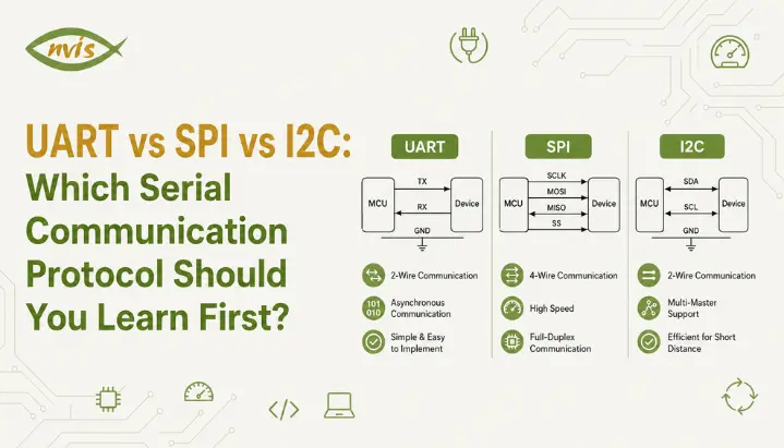
    UART is an acronym for Universal Asynchronous Receiver Transmitter, and because it requires just a few components, it is considered to be an introduction to serial communications into microcontroller circuits. A basic UART connection commonly uses two signal lines, TX and RX, along with a shared ground. Two devices cross connect their transmit and receive lines and share a common ground with the TX pin of one device connected to the RX pin of the other.

    Asynchronous is a key word. There is no special clock wire for UART. Instead, the sending and receiving devices are configured to use the same baud rate in advance. Each device internally uses that agreed setting to determine when to sample each bit, and each device internally uses that speed to time when to sample each bit. Each UART character or frame typically begins with a start bit, followed by the data bits and optional parity bit, and ends with one or more stop bits but, in the absence of a common clock, the receiving UART knows when each byte starts and ends.

    The following is a quick worked example of something which frequently appears in exam-style questions. When the UART is programmed to run at 9600 baud, the time to send one bit is called bit time, and is given by:

    Bit time = 1 / Baud rate = 1 / 9600 = 0.0001042 seconds ≈ 104.2 microseconds

    Let’s assume we’re using a standard 10-bit frame, where each frame contains 1 start bit, 8 data bits, and 1 stop bit, and that we’re sending one whole frame at a time. In this case, the total number of bits is 10, and the time to send one complete frame is about 1.042 milliseconds. Baud-rate and bit-time calculations are useful practice for students studying serial communication and microcontroller timing, and may be relevant to technical-exam questions depending on the exam and syllabus.

    The greatest virtue of UART is its simplicity. It is point-to-point, that is, it connects only two devices – is ideal for debugging via serial monitor, connecting GPS modules or talking to Bluetooth modules such as HC 05. What makes it the least desirable is its point to point character. However, unlike SPI and I2C, UART is difficult to scale to multiple devices on the same bus and if the baud rate is not the same, data is completely garbled.

    SPI: Built for Speed

    Now picture a strict orchestra conductor keeping every musician perfectly in time with a baton. Nobody plays a note unless the conductor’s beat says so, and because everyone follows the same beat, the whole orchestra can play remarkably fast without falling out of sync. SPI works on this same principle of a shared, dedicated timing signal.

    SPI stands for Serial Peripheral Interface, and unlike UART, it is a synchronous protocol, meaning it uses a dedicated clock line so every connected device reads and writes data in perfect step with each clock pulse. The shared clock allows the receiver to sample data at precisely defined clock edges. SPI also has relatively little protocol overhead, which allows many implementations to operate at much higher data rates than typical UART and I2C connections.

    An SPI connection typically uses four lines: MOSI (Master Out Slave In) carries data from controller to peripheral, MISO (Master In Slave Out) carries data back from peripheral to controller, SCK is shared clock line, and SS or CS (Slave Select or Chip Select) tells a specific peripheral device that it is being addressed. Because SPI uses a dedicated select line per device, a single controller can talk to multiple peripherals on the same bus just by toggling which chip select line is active.

    This full-duplex design, combined with low protocol overhead, allows many SPI implementations to operate at several megabits per second or much higher, depending on the microcontroller, peripheral, wiring, and signal integrity. This is exactly why SPI shows up everywhere speed genuinely matters: driving SD cards, refreshing TFT displays, and streaming data from high sample rate sensors like accelerometers.

    The main trade-off is wiring and scalability at the pin level. Every additional SPI peripheral needs its own dedicated chip select line, so a design with many sensors can quickly run out of available microcontroller pins. SPI also has no formal acknowledgment mechanism, so if a peripheral fails to respond, there is no built-in way for the controller to know something went wrong.

    I2C: Many Devices, Few Wires

    Imagine a classroom where the teacher can call out a specific student’s name before asking a question, and every student in the room hears the question but only one called upon responds. Everyone shares the same “wire” of conversation, yet the system stays organized because each student has a unique identity. This is essentially how I2C manages to connect many devices using very few wires.

    I2C, short for Inter Integrated Circuit and often pronounced “I squared C,” is a synchronous serial communication protocol that uses the same two bus lines, SDA and SCL, for multiple connected devices, subject to address availability and electrical bus limitations. These two lines are SDA (Serial Data), which carries actual data, and SCL (Serial Clock), which keeps every device on the bus synchronized to the same timing.

    The mechanism that makes this scalability possible is device addressing. I2C devices can use 7-bit or 10-bit addresses. Although a 7-bit address field provides 128 possible values, some addresses are reserved, and address conflicts can occur when multiple devices use the same fixed address of the specific device it wants to talk to. Every device on a shared bus receives this address, but only the device whose address matches actually responds, similar to the classroom example above. I2C uses 7-bit or 10-bit addressing. Although a 7-bit address field provides 128 possible values, some addresses are reserved, so the number of usable device addresses is lower. In practice, the number of devices is also limited by bus capacitance, address conflicts, and the electrical characteristics of the bus.

    I2C typically operates at up to 100 kbps in standard mode and up to 400 kbps in fast mode, noticeably slower than SPI, and I2C is not full duplex: data is transferred over the shared SDA line, with the controller and target taking turns transmitting according to the bus protocol, even though communication can switch directions when needed. What I2C gives up in raw speed, it makes up for in wiring efficiency, which is why it is widely used in projects involving multiple low-speed sensors, such as temperature sensors, real time clocks, EEPROMs, and accelerometers, all sharing same SDA and SCL lines.

    I2C does have real limitations worth knowing. Because I2C devices use open-drain or open-collector outputs, the SDA and SCL lines are pulled high through external pull-up resistors. Devices actively pull the lines low when transmitting. This arrangement allows multiple devices to share the same bus without directly driving the lines high against one another.

    USB Serial Communication Protocol: How It Connects to UART

    A common point of confusion for beginners is the relationship between UART and USB, especially since the keyword “USB serial communication protocol” often gets searched by people expecting them to be interchangeable. They are related, but they are not the same thing, and understanding differences clears up a lot of confusion when working with development boards.

    When you plug an Arduino or another development board into a laptop over USB, the board may use a USB-to-UART bridge such as a CP2102, CH340, or FTDI device to convert between USB and UART such as a CP2102, CH340, or FTDI device converts USB communication from the computer into UART signals for the microcontroller that microcontroller’s UART actually understands. Your operating system usually shows this connection as a COM port on Windows or a /dev/ttyUSB or /dev/ttyACM device on Linux, even though physically you plugged in a USB cable.

    USB itself is a far more complex, host centric protocol built for plug and play convenience, supporting device enumeration, much higher speeds ranging from 1.5 Mbps in early versions to multiple Gbps in modern versions, and even ability to deliver power to connected devices. UART, by contrast, remains a simple two wire asynchronous protocol running quietly underneath, doing actual byte level framing that your microcontroller’s UART peripheral was built to handle.

    For many development boards, a USB-to-UART bridge connects the computer’s USB interface to the microcontroller’s UART. However, some modern microcontrollers and development boards provide native USB, so USB communication does not necessarily involve UART On boards that use a USB-to-UART bridge, the USB connection provides the computer-side interface while UART handles communication on the microcontroller side you already learned about earlier in this guide.

    UART vs SPI vs I2C: Side by Side Comparison

    ParameterUARTSPII2C
    Full FormUniversal Asynchronous Receiver TransmitterSerial Peripheral InterfaceInter Integrated Circuit
    Clock SignalNone (asynchronous)Yes (synchronous)Yes (synchronous)
    Wires Needed2 (TX, RX)4 (MOSI, MISO, SCK, SS)2 (SDA, SCL)
    Devices Supported2 (point to point)Many, limited by chip select pinsUp to 127+ using addressing
    Typical SpeedUp to 115200 bps commonlyUp to 10 Mbps or higher100 kbps to 400 kbps typically
    Duplex ModeFull duplexFull duplexHalf duplex
    ComplexityLowestModerateModerate to high with multiple devices
    Common Use CaseDebugging, GPS, Bluetooth modulesDisplays, SD cards, high speed sensorsMultiple sensors, EEPROMs, RTCs

    Reading this table, a clear pattern emerges. UART wins on simplicity and is genuinely the easiest serial communication protocol to understand from scratch. SPI wins decisively on speed whenever a project genuinely needs it. I2C wins on wiring efficiency the moment a project grows beyond two or three connected devices. None of them is universally “better,” which is exactly why real embedded systems, from a simple Arduino weather station to a full scale industrial control board, routinely use all three protocols together, each handling part of the job it is best suited for.

    Serial Communication in Microcontroller Projects: Where Each Protocol Fits

    Understanding theory is one thing, but seeing how UART, SPI, and I2C actually show up together inside a real microcontroller project makes choice far more intuitive. Consider a typical IoT weather station built around an ESP32 or Arduino board, a genuinely common beginner project across Indian engineering colleges.

    Many development boards use UART for serial debugging, and some use a USB-to-UART bridge for programming as well. However, some modern boards use native USB or other interfaces for programming, and many development boards provide a serial-monitor connection through USB for convenient debugging. If the project includes a small OLED or TFT display to show live temperature and humidity readings, that display may use SPI, especially when higher data-transfer rates are useful for refreshing the screen, because refreshing a screen quickly benefits enormously from SPI’s higher speed. Meanwhile, actual temperature, humidity, and pressure sensors, such as the BMP280 and many I2C-compatible sensors, are frequently connected over I2C. Some sensors, such as the DHT11/DHT22, use their own single-wire-style communication interface instead, since a project might eventually add two, three, or more sensors, and I2C lets every one of them share same two SDA and SCL wires without consuming extra microcontroller pins.

    This pattern, UART for debugging, SPI for display, I2C for sensors, repeats across an enormous number of real embedded systems in industry, from consumer electronics to automotive dashboards to industrial monitoring equipment. Recognizing this pattern early is far more useful for a beginner than trying to memorize which protocol is “fastest” or “best” in isolation, because in practice, the answer is almost always all three, each doing a different job.

    Which Serial Communication Protocol Should You Learn First?

    If you are a beginner staring at UART, SPI, and I2C for the first time, wondering where to actually start, the honest answer is to learn them in that exact order, and here is the reasoning behind it.

    Start with UART because it has the fewest moving parts. With just two wires and no shared clock to configure, UART lets you focus entirely on core ideas like baud rate, start and stop bits, and asynchronous timing without getting distracted by addressing schemes or multiple chip select lines. Nearly every beginner’s first “real” embedded systems project, printing values to a serial monitor, already uses UART, so you are likely to encounter it naturally within your first week of working with any microcontroller.

    Move to SPI next, once UART feels comfortable. SPI introduces the idea of a shared clock and multiple peripherals through chip select lines, both of which build directly on concepts you already understand from UART, just with an added synchronous twist. Working with an SPI display or an SD card module is a natural next project, and it teaches you why a dedicated clock line matters for speed in a way that reading about it never quite does.

    Finish with I2C, because it is conceptually the most involved of three despite needing fewest wires. Understanding device addressing, half duplex data flow, and how multiple devices share a single bus without colliding is easier to grasp once UART and SPI have already built your intuition for synchronous versus asynchronous communication and for how a controller distinguishes between devices. I2C is also where most beginners start building genuinely multi sensor projects, so having UART and SPI fundamentals already in place makes debugging I2C issues far less frustrating.

    This progression, UART, then SPI, then I2C, is not an arbitrary suggestion. It provides a practical learning progression from simpler point-to-point communication to synchronous and then multi-device bus communication, and it is also a practical order that many beginner-focused embedded systems courses may use, which makes it a genuinely practical study path rather than just a beginner friendly opinion.

    Why This Topic Matters for GATE, SSC JE, and RRB JE Aspirants

    Serial communication concepts can be useful for engineering competitive exams because topics related to microprocessors, microcontrollers, interfacing, and communication may include questions involving data transmission, timing, and interfacing, which makes mastering UART, SPI, and I2C valuable well beyond the lab.

    In GATE Electronics and Communication syllabus, questions on serial communication typically appear under microprocessors and microcontrollers, often testing baud rate calculations, bit time, and framing formats exactly like the worked example covered earlier in this guide. UART timing, baud rate, and bit-time concepts can be useful areas to practice for questions related to microprocessors and microcontrollers.

    For RRB JE Electronics and Communication candidates, the technical section places significant weight on microprocessors, communication engineering, and hardware interfacing topics, all of which draw directly on the same UART, SPI, and I2C fundamentals covered here. SSC JE candidates preparing for the electronics stream face a very similar pattern, with related concepts that may be relevant to the microprocessors, microcontrollers, communication, and electronics topics covered in these examinations, depending on the specific syllabus and paper.

    Beyond direct exam questions, interviewers at PSUs and private embedded companies alike frequently ask candidates to explain practical differences between UART, SPI, and I2C during technical rounds, since it is considered fundamental embedded systems knowledge. Being able to explain not just definitions but why behind each protocol’s design, exactly the approach this guide has taken, tends to stand out far more than a memorized comparison table during an actual interview.

    Career Relevance: Embedded Systems Roles in India

    Serial communication protocols form part of the absolute foundation for embedded systems careers in India, and demonstrating comfort with UART, SPI, and I2C can help candidates perform better in technical interviews and demonstrate practical embedded-systems knowledge at both PSUs and private companies.

    Government and public sector opportunities remain a major draw for many engineering graduates, with organizations like ISRO, DRDO, BEL, and BHEL regularly hiring engineers into roles where embedded hardware knowledge, including serial communication interfacing, is directly tested during technical interviews and sometimes even written exams. These roles typically require qualifying through GATE scores or dedicated PSU recruitment exams, which is exactly why exam relevance covered in the previous section connects so directly to long term career outcomes.

    On the private sector side, embedded systems engineering in India offers a genuinely strong salary trajectory for those who build solid fundamentals early. Entry level embedded engineers typically start in the range of 3 to 8 LPA depending on company and city, with automotive Tier 1 suppliers and semiconductor firms often offering higher end of that range to strong freshers. As experience grows, mid level embedded engineers with 3 to 6 years of experience commonly earn between 8 and 14 LPA, and senior embedded architects at companies working on semiconductors or automotive systems can reach 20 to 35 LPA or beyond, particularly as India’s semiconductor and electric vehicle sectors continue expanding under initiatives like PLI scheme for semiconductor manufacturing.

    Recruiters across this spectrum, from PSUs to automotive companies to pure semiconductor firms, consistently list UART, SPI, and I2C interfacing as baseline expected knowledge for embedded roles, right alongside Embedded C and microcontroller fundamentals. Building genuine hands on familiarity with all three protocols during your college years, rather than memorizing them night before an interview, is one of more reliable ways to stand out early in an embedded systems career.

    Conclusion

    Serial communication protocols might seem like a dense, jargon heavy topic at first glance, but at their core, UART, SPI, and I2C are simply three different answers to the same basic question: how should two or more electronic devices reliably exchange data using as few wires as possible. UART keeps things simple with just two wires and no shared clock, SPI trades extra wiring for serious speed through a dedicated clock line, and I2C sacrifices some speed to let many devices share just two wires through unique addressing.

    If you are just starting out, the clearest path forward is to learn UART first, move to SPI once you are comfortable, and finish with I2C. This order matches how conceptual complexity actually builds across three protocols, and it can provide a practical progression for students learning embedded communication interfaces. Beyond the classroom, this same knowledge directly feeds into GATE, SSC JE, and RRB JE technical sections, and it remains one of most consistently tested fundamentals in embedded systems interviews across PSUs and private companies alike.

    The best way to actually internalize all three protocols is to build something with each of them. Wire up a simple UART serial monitor project this week, add an SPI display next, and connect a couple of I2C sensors after that. Reading about serial communication protocols will only take you so far. Hands on practice is what turns this from exam theory into a skill you genuinely understand.

    FAQs

    UART is asynchronous and needs no shared clock, using just two wires for point to point communication. SPI is synchronous and uses a dedicated clock line along with separate data lines, allowing many implementations to achieve higher data rates than typical UART or I2C configurations. I2C is also synchronous but uses just two shared wires along with device addressing, allowing many devices to communicate over the same bus.

    UART is generally the best starting point because it has fewest moving parts, just two wires and no clock to configure. Once UART feels comfortable, moving to SPI and then I2C builds naturally on concepts already learned, following order of increasing complexity.

    No, USB and UART are related but different. Most microcontroller boards use a small USB to UART bridge chip to convert USB’s packet-based communication into UART signal into simple TX and RX lines that a microcontroller’s UART peripheral actually understands, so the microcontroller may still communicate with the computer through its UART peripheral underneath the USB connection.

    SPI uses a dedicated clock line shared between controller and peripheral devices, so the receiver uses the shared clock edges to determine when to sample data, while UART relies on the agreed baud rate and internal timing to determine when to sample each bit. This synchronous design, combined with full duplex operation over separate MOSI and MISO lines, is what allows SPI to comfortably reach speeds of 10 Mbps or higher in many implementations.

    I2C uses 7-bit or 10-bit addressing, allowing many devices to share the same SDA and SCL lines. The practical number depends on available addresses, address conflicts, bus capacitance, pull-up resistors, and other electrical limitations. In practice, the actual number of devices that work reliably depends on bus capacitance, wire length, and pull up resistor values, so most real projects connect a more modest number of I2C devices.

    Serial communication concepts may be relevant to questions on microprocessors, microcontrollers, communication, and interfacing, depending on the exam and syllabus, often through baud rate and bit time numerical problems. Since these protocols are also fundamental to real embedded systems work, understanding them well serves both exam preparation and practical interview readiness at same time.

    Tags: serial communication protocol, usb serial communication protocol

    Swinburne Test of DC Machine and Its Procedures

    TL;DR

    1. This blog is for electrical engineering students, freshers, and GATE, SSC JE, and RRB JE aspirants who want a clear, practical understanding of the Swinburne test of DC machines and how it is performed in a lab.
    2. Swinburne test is an indirect, no load method used to find efficiency of a DC shunt or compound machine without physically loading it, which saves power and protects large machines from damage during testing.
    3. The core idea is simple: run a machine as an unloaded motor, measure the small amount of power it still draws, treat that as constant loss, and then use this one number to predict efficiency at any load, even full load, without ever applying that load.
    4. The test has real limitations. It ignores rise in iron loss at full load and cannot confirm safe commutation or temperature rise under actual working conditions, so engineers pair it with judgment, not blind trust.
    5. Understanding this test builds foundation for machine testing topics that show up repeatedly in GATE Electrical Engineering, SSC JE, and RRB JE exams, and in real testing lab roles at Indian power sector companies.

    Swinburne’s test is a no load, indirect method used to determine efficiency of a DC shunt or compound machine at any load condition, including full load, without actually connecting that load. Named after Sir James Swinburne, the test is one of earliest and most widely taught techniques in Indian electrical engineering laboratories, and it remains a fixture in both classroom experiments and competitive exam syllabi. This blog explains what Swinburne test of DC machines involves, walks through its circuit and procedure step by step, works through a complete numerical example, and covers where this topic fits into GATE, SSC JE, and RRB JE preparation along with career relevance in India’s power sector.

    Also Read,

    What Is the Swinburne Test of DC Machine, Really?

    Picture a large DC motor at a power plant, something rated at 500 kW. To directly measure its efficiency, you would need to connect a full mechanical load capable of absorbing that much power, plus instruments to measure input and output separately. That kind of setup is expensive, time consuming, and honestly a bit risky for a routine test.

    Swinburne figured out a shortcut. Instead of loading the machine fully, run it as a motor with no load at all. At no load, the machine still draws a small amount of current from supply, just enough to overcome its own internal friction, windage, and core losses. Since there is no mechanical output being delivered, every bit of that input power is going into losses.

    Here is the clever part. Most of these losses, like iron loss, friction, and windage, stay roughly constant whether the machine is lightly loaded or fully loaded, as long as speed and flux stay the same. So if you measure these losses once at no load, you can add them to load dependent copper losses at any current level and calculate efficiency at that load, all without ever connecting a real load. That is the entire logic behind the Swinburne test of a dc machine, and it is why the test is also called a no load test.

    This approach works specifically for DC shunt and level compound machines because their field flux stays practically constant regardless of load. A takeaway worth remembering: Swinburne’s test does not measure efficiency directly, it predicts it using losses measured under a much simpler condition.

    Circuit Diagram and Working Principle

    The test circuit is refreshingly simple compared to what it achieves. A DC shunt machine is connected across a DC supply and runs as an unloaded motor. Two ammeters are placed in circuit, one in main supply line to record total no load current drawn from supply, and one in shunt field circuit to record field current separately. A voltmeter reads supply voltage, and a rheostat in field circuit lets you fine tune speed to machine’s rated value.

    Once connections are made and the motor is running at rated voltage and rated speed with no load on its shaft, three quantities are recorded: supply voltage V, total no load line current I0, and shunt field current Ish. Since field winding and armature are in parallel across supply, current actually flowing through armature at no load is different between two readings.

    No load armature current, Ia0 = I0 minus Ish

    This small no load armature current still causes a copper loss in armature winding, calculated as Ia0 squared multiplied by armature resistance Ra. Everything else the machine draws at no load, that is, input power minus shunt field loss minus this armature copper loss, gets grouped together as constant loss.This constant loss includes iron loss, friction loss, windage loss, and shunt field copper loss. In a shunt machine, the field copper loss remains approximately constant because the field current is nearly constant.

    Constant loss, Pc = V I0 minus (I0 minus Ish) squared multiplied by Ra

    Once a PC is known, you have everything you need. For any load current I want to analyze, new armature current becomes I minus Ish for motoring operation, new armature copper loss is calculated from that current, and adding it to Pc gives total losses at that load. Efficiency then follows from basic input minus losses over input relationship.

    Beginner takeaway: think of Pc as a fixed overhead cost machine pays just to keep spinning, and copper loss as a variable cost that grows with load. Once you know fixed cost, predicting total cost at any load becomes simple arithmetic.

    Step by Step Procedure for Swinburne’s Test

    Running actual experiments follows a fairly disciplined sequence, and Indian engineering labs typically structure it like this.

    DC shunt machine is first connected as per circuit diagram, with ammeters, voltmeter, and field rheostat correctly placed. Before switching on the supply, the field rheostat is kept at minimum resistance to establish maximum field current and adequate flux. The motor is then started using a suitable starter, which limits the high armature current at starting.

    Power is then switched on gradually using a starter, since a DC shunt motor connected directly across full voltage at standstill would draw a dangerously high inrush current. As the motor picks up speed, rheostat is adjusted until the machine reaches its rated speed at rated supply voltage. This step matters because losses being measured are only valid at conditions the machine is designed to run at.

    Once speed stabilizes, readings of supply voltage V, no load line current I0, and shunt field current Ish are noted down from meters. It helps to take these readings two or three times and average them, since small fluctuations in a live circuit are normal.

    Separately, armature resistance Ra is measured using a low voltage DC supply and voltmeter ammeter method, with machine stationary. Since this test cares about performance under working conditions, measured resistance is often corrected to account for temperature rise expected during actual operation, since copper resistance increases with heat.

    With V, I0, Ish, and Ra all recorded, the machine is switched off safely, and the calculation phase begins using formulas covered in the earlier section.

    Worked Numerical Example

    Numbers make this concept click faster than formulas alone, so here is a complete example using values typical of a mid-sized DC shunt motor used in Indian engineering labs.

    Consider a 220 V DC shunt motor with a no load line current I0 of 5 A, a shunt field current Ish of 1 A, and an armature resistance Ra of 0.5 ohm.

    First, find no load armature current. Ia0 = I0 minus Ish = 5 minus 1 = 4 A

    Next, calculate armature copper loss at no load. Armature copper loss = Ia0 squared multiplied by Ra = 4 squared multiplied by 0.5 = 8 watts

    Now calculate no load input power. Input power = V multiplied by I0 = 220 multiplied by 5 = 1100 watts

    Constant loss is calculated by subtracting the no-load armature copper loss from the total no-load input power. Pc = 1100 − 8 = 1092 W. This value includes the shunt field copper loss along with iron, friction, and windage losses.

    This constant loss of 1092 watts is now assumed to hold at any load. Suppose you want to predict a motor’s efficiency when it draws a full load line current of 20 A from supply.

    New armature current at this load: Ia = 20 minus 1 = 19 A New armature copper loss: 19 squared multiplied by 0.5 = 180.5 watts Total losses at full load: Pc plus new armature copper loss = 1092 plus 180.5 = 1272.5 watts Total input at full load: 220 multiplied by 20 = 4400 watts Output power: Input minus total losses = 4400 minus 1272.5 = 3127.5 watts

    Efficiency = Output divided by Input = 3127.5 divided by 4400 = approximately 0.7108, or 71.08 percent

    Notice what just happened. Every single reading in this calculation came from a no load test, yet you now have a full load efficiency figure without ever physically loading the motor to 20 A. That is the practical payoff of the swinburne test.

    Advantages and Limitations of Swinburne’s Test

    Every testing method involves trade offs, and Swinburne’s test is no exception. Being upfront about both sides helps you use test correctly rather than treating it as a universal solution.

    AspectAdvantageLimitation
    Power requirementVery low, since machine runs unloadedCannot verify behavior at high current draw
    Time and setupQuick, minimal equipment, ideal for large machinesRequires a separate resistance measurement step
    Efficiency predictionEfficiency at any load can be predicted from one testAssumes constant losses do not change with load, which is only approximately true
    Iron loss accuracySimple to calculate at no loadArmature reaction increases iron loss at full load, an effect this test ignores
    Commutation and heatingNot applicable hereCannot confirm safe commutation or actual temperature rise under real load
    Machine typeWorks well for shunt and level compound machinesNot usable for series machines, since they cannot run safely at no load

    On the advantage side, the biggest win is the economy. Testing a large machine under full mechanical load, sometimes hundreds of kilowatts, would demand load banks, cooling arrangements, and significant electricity consumption. Swinburne’s test sidesteps all of that by drawing only a fraction of rated power from supply.

    On the limitation side, assumption of constant losses is the test’s biggest weak point. In reality, the armature reaction distorts flux distribution at full load, which pushes iron loss somewhat higher than what was measured at no load, sometimes by a noticeable margin. The test also offers zero insight into commutation quality or winding temperature rise under sustained full load, both of which matter enormously for a machine’s real world reliability. This is exactly why Swinburne’s test is not the final word on a machine’s performance, but rather a fast, economical first estimate.

    Takeaway worth remembering: use Swinburne’s test for quick efficiency prediction and preliminary loss separation, but pair it with a load test or Hopkinson’s test when commutation and thermal behavior genuinely need to be verified.

    Swinburne’s Test vs Hopkinson’s Test vs Brake Test

    Students often confuse Swinburne’s test with other DC machine testing methods taught alongside it. A quick comparison clears this up fast.

    FeatureSwinburne’s TestHopkinson’s TestBrake Test
    Loading methodNo load, indirectTwo machines mechanically coupled, regenerative loadingDirect mechanical loading with a brake
    Power neededVery lowLow, since power is largely recirculated between machinesHigh, full load power actually consumed
    Machines requiredOne machineTwo identical machinesOne machine
    Temperature rise dataNot availableAvailable, since machines run under real load for extended periodsAvailable
    Commutation checkNot possiblePossible under real loadingPossible
    Best suited forQuick efficiency estimate on large shunt or compound machinesDetailed testing of two identical machines togetherSmall machines where direct loading is practical

    Swinburne’s test wins on simplicity and economy. Hopkinson’s test, also called back to back test, addresses temperature and commutation blind spots by actually loading two identical machines against each other, though it needs two machines of same rating, which is not always available. A brake test is the most direct approach but only practical for smaller machines where a mechanical brake can safely absorb power. In an Indian testing lab, all three often appear as separate experiments precisely because each fills a gap others leave open.

    GATE, SSC JE, and RRB JE Exam Relevance

    For students preparing for GATE Electrical Engineering, DC machines carry consistent weightage year after year, and Swinburne test question of dc machine shows up frequently as a numerical problem rather than a purely theoretical one. Typical question patterns ask you to calculate constant loss from given no load readings, then use that to find efficiency at a specified full load current, exactly the kind of calculation walked through in the numerical example above. Getting comfortable with algebra of Ia0 = I0 minus Ish and constant loss formula pays off directly in exam scoring.

    SSC JE and RRB JE electrical papers tend to test this topic at a slightly more conceptual level, often through objective questions on why the test cannot be used for series machines, what constant loss physically represents, or which losses test assumes remain unchanged with load. Since these exams favor concise, accurate recall over multi step derivations, understanding reasoning behind each formula, not just memorizing it, tends to serve candidates better than rote learning.

    Both exam tracks also occasionally test comparison between Swinburne’s test, Hopkinson’s test, and direct loading, so table earlier in this blog doubles as solid revision material. A beginner friendly takeaway here: exam setters love this topic because it rewards genuine understanding over memorization, so working through a few numericals yourself, similar to example above, is more useful than reading formulas passively.

    Career Relevance in India’s Power and Electrical Testing Sector

    Beyond exams, the Swinburne test reflects a habit of thinking that Indian electrical engineers use throughout their careers, which is predicting performance efficiently rather than testing everything in an expensive, time consuming way. Testing and quality roles at PSUs like BHEL, NTPC, and Power Grid Corporation regularly involve exactly this kind of no load and indirect testing on motors and generators before they are commissioned into service.

    Beyond exam preparation, the concepts learned through DC machine testing can also support careers in electrical testing, maintenance, manufacturing, and power engineering. For students, the practical value of the Swinburne test lies more in building an understanding of machine losses, efficiency, and testing methods than in directly qualifying for a particular job Junior Engineer and Assistant Engineer positions filled through SSC JE and RRB JE follow 7th Pay Commission structure, generally starting around 35,400 rupees basic pay at Junior Engineer level, rising to higher pay bands at Assistant Engineer level, with gross monthly salaries commonly falling between 50,000 and 90,000 rupees once allowances are included.

    Private sector opportunities have expanded meaningfully too, particularly in India’s growing renewable energy and EV manufacturing space, where power electronics and motor testing skills, the same fundamentals built through experiments like the Swinburne test, are in strong demand. Engineers with hands-on testing experience and machine fundamentals often find these concepts directly applicable when evaluating motor efficiency for EV drivetrains or industrial automation systems. A solid grip on foundational DC machine testing, in other words, keeps paying dividends well beyond exam hall.

    Conclusion

    Swinburne test of DC machine solves a genuinely practical problem: how do you find a large motor’s efficiency without cost and risk of loading it fully? By running a machine unloaded, measuring its small no load losses, and treating those losses as roughly constant across load conditions, the test lets you predict efficiency at any load, including full load, using just a handful of simple readings. The method is fast, economical, and easy to set up, which explains why it remains a staple experiment in Indian electrical engineering labs and a recurring topic in GATE, SSC JE, and RRB JE exams.

    At the same time, its assumptions have real boundaries. Iron loss does shift under full load due to armature reaction, and the test tells you nothing about commutation quality or temperature rise under sustained operation, which is why it works best as a quick first estimate rather than a complete performance certificate. Understanding both what the test reveals and what it deliberately leaves out is what separates rote memorization from genuine engineering judgment, and that judgment is exactly what shows up in exam numericals and real testing lab work alike. If you are preparing for GATE or a JE exam, work through a few more numericals on your own using different no load readings until calculation feels automatic rather than memorized.

    FAQs

    Swinburne test is used to determine efficiency of a DC shunt or compound machine at any load, including full load, by measuring its losses at no load and using that data to predict performance under loaded conditions without physically applying that load.

    A DC series motor cannot run safely at no load because its speed would rise to dangerously high, potentially damaging levels without a load to hold it in check, and since Swinburne’s test requires a running machine unloaded, it simply cannot be applied to series machines.

    Constant loss in the Swinburne test includes iron losses, friction and windage losses, and shunt field copper loss. These are treated as approximately constant when the machine operates at nearly constant voltage, speed, and flux.

    Armature copper loss is calculated by squaring armature current and multiplying it by armature resistance, written as Ia squared multiplied by Ra, using no load armature current for initial constant loss calculation and load specific armature current for efficiency at any given load.

    The test assumes constant losses remain unchanged from no load to full load, which is not entirely accurate since armature reaction increases iron loss under load, and it also cannot verify safe commutation or actual temperature rise during sustained full load operation.

    Yes, Swinburne’s test appears regularly in GATE Electrical Engineering as numerical problems involving efficiency calculation, and in SSC JE and RRB JE papers as conceptual questions on constant loss and machine applicability, making it a consistently high value topic across these exams.

    Best LCR Meter Features Every Lab Should Look For

    TL;DR –


    • This guide is designed for electronics engineers, lab managers, quality control teams, R&D professionals, and educational institutions looking to choose the right LCR meter for accurate and reliable component testing.
    • LCR meters are essential lab instruments used to measure inductance, capacitance, and resistance, enabling component validation, quality control, R&D, and failure analysis.
    • Compared to basic multimeters, digital LCR meters offer higher accuracy, AC testing at real-world frequencies, automation, and advanced analysis capabilities.
    •  Accuracy, wide test frequency range, programmable test voltage, fast measurement speed, advanced parameters (ESR, impedance, phase angle), and stable readouts are critical for dependable results.
    • The best LCR meter depends on lab needs,high accuracy and advanced features for R&D, speed and repeatability for quality control, and ease of use and durability for educational labs.


    Modern electronics laboratories,whether focused on R&D, quality control, manufacturing, or education,rely heavily on precise component testing. LCR meters are one of the most important tools in this ecosystem. They are used to measure inductance (L), capacitance (C) and resistance (R), the basis of characterizing components, troubleshooting, and compliance testing.

    Labs can no longer depend on simple instruments as components are smaller, tolerances are tight, and the requirements of the application increase. In particular, the digital LCR meters have changed the way the engineers and technicians would measure, analyze and document the results.However, the wide range of available models and specifications can make selecting the right LCR meter challenging.

    Key features of modern LCR meters,such as surface-mount design, large LCD displays, and advanced measurement technology,make them easy to operate, visually refined, and well suited for production-line quality control, incoming component inspection, and automated test systems.

    Related Blogs: 

    Understanding LCR Meters and Their Role in the Lab

    Before diving into features, it’s important to understand what LCR meters actually do and why they are essential.

    An LCR meter is a precision test instrument designed to measure:

    • Inductance (L) of coils and inductors
    • Capacitance (C) of capacitors
    • Resistance (R) of resistors and other components

    LCR meters use AC test signals at specific frequencies, unlike basic multimeters.This will enable them to test the behavior of components at operating conditions in the real world and not only in the case of DC measurements.

    Why Labs Depend on LCR Meters

    • Component validation: Ensuring parts meet design specifications
    • Quality control: Detecting faulty or out-of-tolerance components
    • R&D: Characterizing new materials and designs
    • Failure analysis: Identifying degradation, drift, or defects

    In modern environments, digital LCR meters have become the standard because they offer higher accuracy, automation, and advanced analysis capabilities.

    Types of LCR Meters

    LCR meters using a DC based approach to determine capacitance using the RC time constant, including handheld DMMs with capacitance measurement, have a typical accuracy of approximately ±1% of their capacitance. Handheld digital LCR meters are portable and convenient, making them suitable for on-site testing and field maintenance. Benchtop LCR meters typically offer programmable test rates, high measurement accuracy (often up to 0.01%), computer control, and advanced automation features and are commonly used in calibration, dielectric measurements, and high volume production testing.

    1-Test Frequency

    Electronic elements have to be tested with frequencies that are similar to results in field operations. LCR meters featuring a wide frequency range and frequency selection which can be programmed give the versatility required by both production and research applications.

    Frequencies used commonly are 50/60 Hz, 120 Hz, 1 kHz, 100 kHz and 1 MHz. Programmable-frequency instruments enable users to adjust test settings to real applications or to characterize frequencies in R&D systems to determine suitable operating frequencies and identify potential resonances. In the majority of modern LCR meters, an AC test signal is used and has frequency ranges around 10 Hz to 2 MHz.

    2- Test Voltage

    Most LCR meters permit AC test voltage to be programmed so that the users can regulate the signal level applied to the DUT. The given output voltage is usually determined under the open-circuit conditions.

    There is a source resistance internally, and series connected with the AC output and this yields a voltage drop when a device is connected. As a result, the actual voltage applied to the DUT depends on both the meter’s internal source resistance and the impedance of the component under test.

    3- Accuracy and Measurement Speed

    LCR measurements are necessarily associated with accuracy and speed of measurement. Greater accuracy implies that the measurement times are usually increased whereas faster measurements can limit precision. In order to overcome this trade-off, most LCR meters provide a variety of measurement speed options – often slow, medium and fast.

    Depending on the need of the DUT, users have the opportunity of choosing the right mode. Other features that may be used to improve accuracy include averaging and median filtering but these increase the time of the measurements. Specifications of accuracy should be checked in the instrument manual because the general measurement accuracy depends on the frequency, the test voltage and the DUT impedance.

    4- Measurement Parameters

    Although inductance ( L ), capacitance ( C ), and resistance ( R ) are the most important parameters of measurement, they do not completely describe passive components. Secondary parameters like conductance (G), susceptance (B), phase angle (θ) and equivalent series resistance (ESR) are more insightful into the electrical performance of parts, sensors and materials.

    LCR Meter Features Every Lab Should Look For

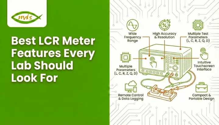
    • Large LCD with backlight: Ensures clear visibility of measurements, even in low-light lab environments.
    • Easy operation with strong functions: Allows users to perform accurate measurements quickly without complex setup.
    • SMT surface-mount technology: Improves durability, reliability, and overall instrument performance.
    • Fast measurement speed (80 ms): Enables quick testing, increasing efficiency in production and quality control.
    • Good readout stability: Delivers consistent and repeatable measurement results.
    • Dual output impedance (30 Ω, 100 Ω): Provides flexibility to match different components and testing requirements.

    Core LCR Meter Capabilities Every Lab Should Look For

    The LCR meter that should be sought by every laboratory should be able to give precise and consistent measurements of inductance, capacitance and resistance elementary in order to have trustworthy component testing. It ought to be operated with an AC test signal over appropriate frequencies to enable components to be tested in realistic working conditions as opposed to DC tests. Easy display readability, measurement stability, and high response time are needed to enable effective daily testing.

    Moreover, the current digital LCR meters are expected to have convenient design and include technical options, like programmable frequencies, automation, and connection to the data. These features assist the laboratories in simplifying the quality control, enhance the productivity, and also aid in the advanced research, thus the LCR meter is also a necessary tool in the R&D, production, and inspection units.

    Measurement Accuracy and Precision

    Accuracy is the single most important feature to evaluate when selecting LCR meters.

    Why Accuracy Matters

    Even small measurement errors can lead to:

    • Incorrect design decisions
    • Component mismatches
    • Product failures in the field

    High-quality LCR meters specify accuracy as a percentage of reading plus counts. For professional labs, higher accuracy directly translates to confidence in results.

    What to Look For

    • High base accuracy across L, C, and R measurements
    • Excellent repeatability
    • Minimal drift over time

    Digital LCR meters typically outperform analog models by providing consistent, repeatable results with minimal operator influence.

    Support for Advanced Measurement Parameters

    Basic measurements of inductance, capacitance and resistance are necessary but within most laboratories more detailed understanding of the behavior of the components is needed. More detailed electrical characterization of components is given by such advanced measurement parameters as equivalent series resistance (ESR), DC resistance (DCR), impedance and admittance and phase angle with dissipation factor.

    The parameters are particularly important when working with power electronics, high-frequency circuits and reliability, when the performance in different conditions should be accurately measured. Digital LCR meters with high end features are able to show more than just one parameter at a time and assist the lab to save time and increase efficiency, as well as provide a more analytical insight.

    Connectivity, Automation, and Data Management

    There is hardly a case when modern labs work independently. Automated test systems commonly include instruments, which are linked with lab management systems.

    Essential Connectivity Options

    • USB for local data transfer
    • LAN for network integration
    • GPIB for legacy automated systems

    Benefits of Connectivity

    • Automated testing and control
    • Seamless data logging
    • Easy report generation and traceability

    Digital LCR meters with strong connectivity options are ideal for labs aiming to scale operations or comply with documentation standards.

    LCR Meter Calibration Stability and Maintenance

    The stability of the calibration is a very important aspect of long-term accuracy and reliability of LCR meters. A stable instrument has the same performance over time in terms of measurements and decreases the number of recalibrations and downtimes. Good digital LCR meters have their internal reference components that are stable and designed in a way that they enable these meters to maintain their accuracy even when in constant use.

    LCR meters require proper maintenance and frequent calibration to ensure their operation within a given range of tolerances. The ability to perform easy calibration processes, clear documentation, and long calibration intervals also allow laboratories to stay in line with quality standards and reduce maintenance effort and operational costs.

    Matching LCR Meter Features to Lab Applications

    Not every laboratory has the same testing needs and the best LCR meter will be highly dependent on what it is going to be used for. Appropriate choice of features depending on usage will provide correct results, efficient workflows and better return on investment.

    The R&D Labs typically need LCR meters with a broad frequency range, which are able to support higher-level parameters of measurement and a high level of accuracy so that a detailed characterization of the components and experimental studies can be provided.

    The advantages of Quality Control Labs include high-speed measurements, high repeatability and strong data logging and reporting options to facilitate large-scale testing and regular inspection procedure.

    Educational Labs are designed with ease of use, tough construction and simplicity of displaying results so that students need not spend much time in training and wear and tear of measurement equipment.

    Knowing exactly what you will use is one of the ways that you can be certain that you are choosing the LCR meters that will provide the optimal mix of performance, usability and cost without being too complicated or too cheap.

    Conclusion:

    The choice of the appropriate instrument is not about specifications but rather about the correspondence between the features and the real-life requirements. LCR meters are very important in determining quality of the product, accuracy of design and efficiency of operation.

    Accurate measurement, frequency range, sophisticated settings, usability and connectivity can make labs comfortably select digital LCR meters that provide reliable and stable performance presently and flexibility in the future.

    Choosing the right LCR meter is not just an equipment purchase,it’s a commitment to precision, efficiency, and excellence in laboratory work.

    FAQs

    An LCR meter is used to measure inductance, capacitance, and resistance of electronic components for testing, quality control, and research purposes.

    Digital LCR meters provide higher accuracy, faster measurements, and advanced features that help labs test components more efficiently and reliably.

    A good LCR meter should support a wide frequency range so components can be tested under real operating conditions.

    In addition to L, C, and R, LCR meters can measure ESR, impedance, phase angle, and dissipation factor for deeper component analysis.

    Choose an LCR meter based on your lab’s needs-accuracy and advanced features for R&D, speed and repeatability for quality control, and ease of use for education labs.

    Tags: Digital LCR meter, LCR meter

    LCR Meter Working Principle: How Inductance, Capacitance & Resistance Are Measured

    TL;DR –

    • This blog is written for electronics students, engineers, lab technicians, manufacturers, educators, and repair professionals who need accurate measurement of inductance, capacitance, and resistance in real-world applications.
    • An LCR meter measures L, C, and R by applying a known AC test signal and analyzing impedance, voltage, current, and phase angle instead of relying on simple DC measurement.
    • The lcr meter working principle is based on impedance analysis, where resistance and reactance (from inductance or capacitance) are separated using phase relationships.
    • By detecting whether current leads, lags, or stays in phase with voltage, the meter accurately identifies and calculates capacitance, inductance, or resistance values.
    • The digital LCR meter working principle improves accuracy and speed through digital signal processing, auto-ranging, and frequency selection, making it ideal for modern labs, R&D, and quality control.

    Related Blogs –


    An LCR meter is a sensitive instrument used to measure inductance (L), capacitance (C), and resistance (R) by applying an AC test signal and analyzing impedance, phase angle, voltage, and current. Understanding the LCR meter working principle enables engineers, technicians, students, and manufacturers to obtain accurate component measurements for testing, design, quality control, and troubleshooting. Precision is important whether you are testing a capacitor on a PCB, checking an inductor in a power supply, or verifying resistor tolerances in a production process.

    A LCR meter is a type of meter created to measure passive components with significantly higher precision than any ordinary multimeter. Although a multimeter can measure the value of resistance and approximately determine the value of capacitance, it cannot analyze frequency-dependent behavior or phase relationships, both of which are required of inductors and capacitors.

    What Does an LCR Meter Measure?

    We will discuss the working principle but first, it would be appropriate to take a quick review of the three parameters measured.

    Inductance (L)

    Resistance to varying currents in a magnetic field by storing energy in a component (usually a coil) is known as inductance. It is expressed in henries (H), and very frequency-dependent.

    Capacitance (C)

    The capacity of a component to store electrical energy in an electric field is called Capacitance. It is expressed in farads (F) and it depends on the frequency, temperature and dielectric material.

    Resistance (R)

    Resistance is the opposition to the flow of electric current and is expressed as ohms (Ω). Resistance is theoretically frequency-independent, in contrast to inductance and capacitance, but in practice, components exhibit parasitic effects.

    All three are measured on an LCR meter, which measures the behavior of a component when it is exposed to an AC signal.

    The LCR Meter Working Principle

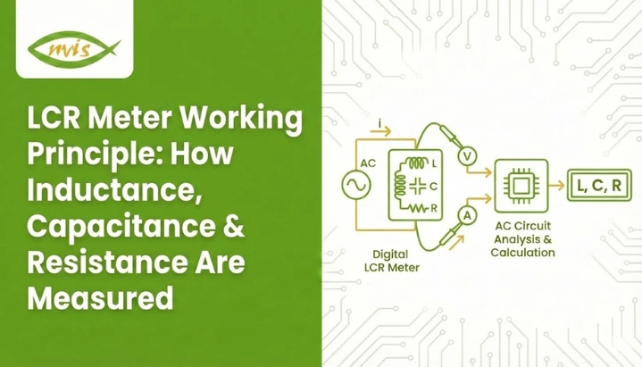
    LCR meter working principle is based on measuring the impedance of a component when it is excited by a known AC test signal. Measuring the reaction of the component to this signal, that is, the value of both voltage and current, and the angle between them, the meter will precisely decide whether the component is a resistor, capacitor, or inductor, and compute its value.

    The principle of working of the LCR meter is impedance measurement which enables the instrument to analyze the response of a component to an alternating current (AC) signal.

    Impedance (Z) is the total opposition a circuit presents to alternating current. Unlike simple resistance in DC circuits, impedance consists of resistance (R) and reactance (X).

    • Resistance (R)
    • Reactance (X) from inductance or capacitance

    The fundamental relationship is:

    • Inductive reactance: XL = 2πfL
    • Capacitive reactance: XC = 1 / (2πfC)

    By applying a known AC signal and measuring:

    • Voltage (V)
    • Current (I)
    • Phase angle (θ) between them

    The LCR meter establishes whether the component is mostly a resistor, capacitor or inductor and calculates it.

    Nvis 9303T Digital LCR Meter – Overview

    The Nvis 9303T is a digital LCR meter designed for accurate measurement of passive electronic components like inductors (L), capacitors (C), and resistors (R). It’s typically used in quality control, incoming inspection of components, and automated test systems in industrial and laboratory environments. 

    Parameter

    Frequency

    Typical Range (example)

    Capacitance (C)

    1 kHz

    0.1 pF – 9999.9 pF


    10 kHz

    0.01 pF – 999.99 pF

    Inductance (L)

    1 kHz

    0.1 pH – 9999.9 H


    10 kHz

    0.01 pH – 999.99 H

    Dissipation / Quality

    All

    D: 0.0001 – 9.999, Q: 0.0001 – 9999


    How an LCR Meter Works: Step-by-Step

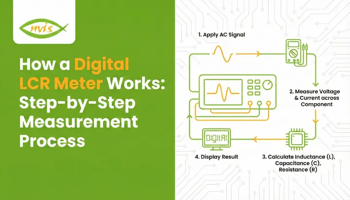
    When the lcr meter working process is divided into a logical sequence the process becomes much clearer. Each step is based on the LCR meter working principle of AC impedance measurement and phase analysis.

    1 AC Signal Generation

    The LCR meter generates a stable AC test signal using an internal oscillator. Common test frequencies include:

    • 100 Hz
    • 120 Hz
    • 1 kHz
    • 10 kHz
      Some advanced meters offer selectable or automatic frequency ranges.

    2 Applying the Test Signal to the Component

    The component under test (DUT) is connected using:

    • Two-terminal method (basic measurements)
    • Four-terminal (Kelvin) method for higher accuracy

    The four-terminal method eliminates errors caused by lead resistance and contact impedance.

    3 Measuring Voltage and Current

    Precision circuits inside the meter measure the voltage across and current through the component. These measurements form the basis of impedance calculation.

    4 Phase Angle Detection

    The phase difference between voltage and current reveals the component type:

    • 0° phase shift – Pure resistance
    • Current leads voltage – Capacitive behavior
    • Current lags voltage – Inductive behavior

    5 Parameter Calculation and Display

    Using digital signal processing, the meter calculates L, C, or R and displays the value on the screen, often along with:

    • Quality factor (Q)
    • Dissipation factor (D)
    • Equivalent series resistance (ESR)

    How Inductance, Capacitance & Resistance Are Measured

    An LCR meter is an inductance, capacitance, and resistance meter that uses the same basic principle, which is the analysis of AC impedance, but presents the results differently, based on the behavior of the component to the signal applied to it. In this section, the extracting principle of each parameter is detailed according to the lcr meter working principle.

    How Resistance (R) Is Measured

    When a purely resistive component is tested:

    • Voltage and current remain in phase (0° phase angle)
    • There is no reactive component (no energy storage)
    • Impedance is equal to resistance

    The LCR meter calculates resistance using:

    • R = V / I

    The meter uses an AC signal even in measuring resistance. This enables it to sense parasitic inductance or capacitance which a DC multimeter would not, and makes the measurement more realistic of actual parts.

    How Capacitance (C) Is Measured

    For capacitors, the current leads the voltage, creating a negative phase angle.

    Measurement process:

    • The meter applies a known AC frequency
    • It measures voltage, current, and phase angle
    • Capacitive reactance is calculated:
      • XC = 1 / (2πfC)

    From this relationship, the meter computes capacitance:

    • C = 1 / (2πfXC)

    Since the capacitance depends on the frequency and dielectric losses, the LCR meters can be configured to use realistic and application relevant frequencies (usually 100 Hz or 1 kHz).

    How Inductance (L) Is Measured

    For inductors, the current lags behind the voltage, producing a positive phase angle.

    Measurement process:

    • The AC signal causes energy storage in a magnetic field
    • Inductive reactance is calculated:
      • XL = 2πfL

    The meter then determines inductance:

    • L = XL / (2πf)

    Higher test frequencies are often used to improve sensitivity, especially for small inductance values.

    Why This Measurement Method Matters

    By gauging the behavior of a component under AC conditions, an LCR meter provides:

    • More realistic values than DC testing
    • Higher accuracy for frequency-sensitive components
    • Reliable data for quality control, testing, and design

    Inductance, capacitance, and resistance are measured by observing how voltage and current interact under AC excitation, making the LCR meter an essential tool for precise electronic component analysis.

    Accuracy Factors in LCR Measurement

    Even the best LCR meter requires proper usage to achieve accurate results.

    Common Influencing Factors

    • Test lead length and quality
    • Stray capacitance and inductance
    • Component temperature
    • Calibration status

    High-end meters include open, short, and load compensation to eliminate systematic errors.

    Analog vs Digital LCR Meter Working

    Feature

    Analog LCR Meter

    Digital LCR Meter

    Accuracy

    Moderate

    High

    Ease of use

    Manual balancing

    Automatic

    Measurement speed

    Slow

    Fast

    Data display

    Scale-based

    Numeric + parameters

    Modern usage

    Limited

    Industry standard

    Due to efficiency and precision, digital models dominate today’s laboratories.

    Conclusion

    The working principle of an LCR meter is based on a simple yet powerful concept, which involves using a known AC signal and observing the response of a component. Through impedance and phase relation measurements, an LCR meter can accurately measure inductance, capacitance, and resistance, which are important parameters in modern electronics.

    Understanding the principles of lcr meter working is not only going to enhance the accuracy of measurements, but also assist the user to identify the correct instrument to use, prevent certain mistakes, and analyze the results properly. With the further development of electronics, tthe digital LCR meter working principle enables faster, smarter, and more reliable component testing of components in education, industry and research.

    FAQs

    An LCR meter is a device that uses a known AC test signal applied to a component and measures the impedance of the component which is the voltage, current and the phase angle. Based on these values, the meter determines whether the component behaves as a resistor, capacitor, or inductor and calculates its precise value.

    Inductance and capacitance are its frequency-dependents that cannot be accurately measured by DC. The AC signal enables the LCR meter to measure reactance and phase shift that is needed to calculate the values of L and C.

    The series mode applies in cases where resistive losses are the most important (usually when the inductance is small and the capacitors of interest are very low-value), whereas the parallel mode is used where leakage losses or parallel resistance are important (large capacitors).

    Since reactance varies with frequency, capacitor and inductor impedance vary with the test frequency. The loss and material properties also change with the frequency, which interferes with the measurement outcomes.

    Yes. An LCR meter measures resistance under AC impedance, and therefore is able to take into consideration parasitic inductance and capacitance which cannot be sensed in a DC multimeter, leading to further refined measurements of actual components.

    Tags: digital lcr meter working principle, lcr meter working, lcr meter working principle

    Gauss Meter Is Used to Measure What? Magnetic Field Explained

    TL;DR –

    • This blog is written for electronics engineers, technicians, students, educators, R&D professionals, and quality control teams who need a clear understanding of magnetic field measurement.
    • It explains what a gauss meter is used to measure, focusing on magnetic field strength and magnetic flux density in gauss or tesla units.
    • The blog breaks down gauss meter measurement principles, including how sensors and probes detect static (DC) and alternating (AC) magnetic fields.
    • It highlights real-world applications of gauss meters in electronics testing, magnet manufacturing, automotive systems, medical equipment, and research labs.
    • The blog emphasizes accuracy, proper usage, and correct selection of gauss meters to ensure reliable, safe, and consistent magnetic field measurements.

    Magnetic fields play a critical role in modern technology, even though they are invisible to the human eye. From smartphones, electric vehicles, and power supplies to medical equipment and industrial machinery, magnetic fields influence performance, safety, and reliability. Measuring these fields accurately is essential to ensure devices work as intended and comply with design standards.

    This is where a gauss meter becomes important. Many engineers, students, and technicians ask a simple but fundamental question: gauss meter is used to measure The answer lies in understanding magnetic field strength and how it affects electrical and electronic systems.

    In this detailed guide, we will explain gauss meter measurement, what a gauss meter is used to measure, how it works, its types, applications, and best practices. By the end of this blog, you will have a clear, practical understanding of magnetic field measurement and why gauss meters are indispensable tools across industries.


    Related Blogs


    What Is a Gauss Meter?

    A Gauss meter is a scientific and electronic measurement instrument used to measure the strength and direction of a magnetic field. It measures magnetic flux density, typically expressed in Gauss (G) or Tesla (T), where 1 Tesla = 10,000 Gauss.

    Gauss meters are widely used in electronics labs, physics experiments, industrial testing, research, and education to analyze magnetic fields generated by permanent magnets, electromagnets, motors, transformers, and electronic components.

    The unit of measurement used by a gauss meter is typically gauss (G) or tesla (T):

    • 1 tesla = 10,000 gauss
    • Gauss is commonly used for lower-strength magnetic fields
    • Tesla is used for very strong magnetic fields, such as in MRI systems

    When people ask gauss meter is used to measure what, the most accurate answer is:

    A gauss meter is used to measure the strength and sometimes the direction of magnetic fields.

    Understanding Magnetic Fields Measurement  

    A magnetic field is an invisible force field that surrounds magnets, electric currents, and changing electric fields. It represents the region where magnetic forces can be detected and measured. Magnetic fields are fundamental to how many electrical and electronic systems operate, from simple motors to advanced medical and industrial equipment.

    Magnetic fields are described by their strength and direction. Strength indicates how intense the field is at a given point, while direction shows the orientation of the magnetic force. These characteristics are commonly visualized using magnetic field lines, which emerge from the north pole of a magnet and enter the south pole. The closer the lines, the stronger the magnetic field.

    The key quantity used to describe magnetic field strength is magnetic flux density, measured in gauss (G) or tesla (T). This is precisely what instruments like gauss meters are designed to measure. Understanding magnetic fields and their behavior is essential for designing reliable electronics, ensuring safety, and maintaining consistent performance in real-world applications.

    What Does a Gauss Meter Measure?

    A gauss meter is a precision measurement instrument used to evaluate magnetic fields with high accuracy. It plays a critical role in electronics, electrical engineering, physics laboratories, manufacturing, and quality control, where understanding magnetic behavior is essential for performance, safety, and reliability.

    A gauss meter is designed to measure the strength and characteristics of a magnetic field. Its primary measurements include:

    • Magnetic field strength
      This indicates how strong the magnetic field is at a specific point. It is typically expressed in Gauss (G) or Tesla (T) and helps determine whether a magnetic source meets required specifications.
    • Magnetic flux density
      Magnetic flux density describes how concentrated the magnetic field lines are in a given area. This measurement is especially important in applications involving motors, transformers, and magnetic sensors, where field uniformity directly affects efficiency and performance.
    • Field polarity and direction
      Many modern gauss meters can identify whether the magnetic field is north or south oriented and detect its direction. This is crucial when aligning magnets, testing assemblies, or verifying correct installation in electromechanical systems.

    Static and Dynamic Magnetic Fields

    Depending on its design and sensor type, a gauss meter can measure both:

    • Static (DC) magnetic fields – typically produced by permanent magnets
    • Alternating (AC) magnetic fields – generated by coils, motors, and power systems

    Understanding whether the magnetic field is AC or DC is crucial for accurate gauss meter measurement and correct data interpretation, especially in diagnostics, quality control, and research applications.

    How Gauss Meter Measurement Works

    A gauss meter measures magnetic fields by detecting how a magnetic force influences an electronic sensor and converting that influence into a readable numerical value. The measurement process is designed to be precise, repeatable, and suitable for both laboratory and industrial environments.

    Sensor Principle

    Most modern gauss meters operate using a magnetic field sensor placed inside a probe. When the probe is exposed to a magnetic field, the sensor converts the magnetic signal into an electrical signal.

    Probe Orientation

    One of the most important factors in accurate gauss meter measurement is probe orientation. Magnetic fields have direction, and incorrect alignment can lead to inaccurate readings. Advanced gauss meters may use multi-axis probes to capture field strength in different directions simultaneously.

    Display and Output

    Digital gauss meters provide:

    • Instant readings on an LCD screen
    • High resolution and repeatability
    • Data logging and computer connectivity in advanced models

    Types of Gauss Meters

    Different applications demand different levels of accuracy, functionality, and field analysis. Understanding the types of gauss meters helps engineers, technicians, educators, and students select the right instrument for accurate magnetic field measurement.

    • Digital Gauss Meters

    Offer high accuracy, fast response, and an easy-to-read digital display. Widely used in laboratories, R&D, and industrial testing.

    • Analog Gauss Meters

    Based on older technology with limited accuracy. Mostly replaced by digital gauss meters in modern applications.

    • Single-Axis Gauss Meters

    Measure magnetic fields in one direction. Suitable for basic and routine magnetic field testing.

    • Three-Axis Gauss Meters

    Measure magnetic fields in X, Y, and Z directions, making them ideal for complex and non-uniform magnetic field environments.

    Why Accuracy Is Critical in Gauss Meter Measurement

    Accurate gauss meter measurement is essential because even minor errors in magnetic field readings can lead to serious technical and safety problems. Magnetic fields directly influence how electronic and electromechanical systems behave, and incorrect measurements can compromise performance, reliability, and compliance.

    In electronics, excess or uncontrolled magnetic fields can:

    • Interfere with sensitive circuits and signal integrity
    • Cause sensor malfunction or inaccurate feedback
    • Lead to overheating, efficiency loss, or premature component failure

    Precise gauss meter measurements help engineers identify and control these risks during design, testing, and quality assurance.

    Importance of Precision in Magnetic Field Measurement

    Accurate readings ensure:

    • Reliable and consistent product performance
    • Safety of equipment and users, particularly in high-power or industrial environments
    • Compliance with design specifications and industry standards, reducing rework and failures

    To maintain high accuracy, gauss meters must be properly calibrated, used with correct probe alignment, and operated under recommended measurement conditions. This disciplined approach ensures dependable magnetic field data across laboratories, manufacturing floors, and research environments.

    Gauss Meter vs Other Magnetic Field Measurement Tools

    Different tools are used to measure magnetic fields, but each serves a specific purpose. Understanding how a gauss meter compares with other magnetic field measurement instruments helps in selecting the right tool for the job.

    Tool

    What It Measures

    Best For

    Key Characteristics

    Gauss Meter

    Magnetic field strength in Gauss or Tesla

    Permanent magnets, motors, transformers, electronic assemblies

    High accuracy, fast response, ideal for lab and industrial testing

    Teslameter

    Magnetic field strength in Tesla

    Strong magnetic fields, research, high-power applications

    Similar to gauss meter but optimized for high-field measurements

    Search Coil Sensors

    Changing (AC) magnetic fields

    Dynamic magnetic field analysis

    Works on electromagnetic induction; not suitable for static (DC) fields

    Fluxgate Magnetometers

    Very weak magnetic fields

    Geophysics, navigation, Earth’s magnetic field studies

    Extremely sensitive; not commonly used for routine electronics testing


    Conclusion

    To summarize, a gauss meter is used to measure magnetic field strength or magnetic field, providing critical insights into how magnetic fields behave in real-world systems. From electronics and automotive engineering to healthcare and research, gauss meter measurement ensures accuracy, safety, and performance.

    Understanding what a gauss meter measures, how it works, and how to use it correctly empowers engineers, technicians, and students to make informed decisions and reliable measurements. As technology continues to advance, the gauss meter will remain a fundamental tool for exploring and controlling the invisible force of magnetism.


    FAQs

    A gauss meter is used to measure the strength of a magnetic field, specifically magnetic.It shows how strong a magnetic field is at a particular point, usually in gauss or tesla units.

    Gauss meter measurement means checking how strong a magnetic field is around a magnet, electrical device, or component, helping ensure safe operation and correct performance.

    Yes, many modern gauss meters can measure both DC magnetic fields from permanent magnets and AC magnetic fields produced by coils, motors, and power systems.

    Gauss meter measurement is widely used in electronics testing, magnet manufacturing, automotive and EV systems, medical equipment monitoring, and research laboratories.

    A gauss meter helps detect unwanted or excessive magnetic fields that can interfere with electronic circuits, sensors, and components, ensuring reliability and safety.

    Tags: gauss meter is used to measure, gauss meter measurement

    How a Digital LCR Meter Works: Step-by-Step Measurement Process

    TL;DR –

    • This blog is written for electronics engineers, technicians, students, educators, and R&D professionals who want a clear, practical understanding of how a digital LCR meter works.
    • The blog explains what a digital LCR meter is and why it is essential for accurate measurement of inductance, capacitance, and resistance.
    • It breaks down the digital LCR meter working principle, showing how AC signals, phase measurement, and impedance calculation are used.
    • The blog covers measurement modes, test frequency importance, and common mistakes to ensure accurate results.
    • It highlights real-world applications and advantages of using an LCR meter digital instrument in labs, manufacturing, and education.


    Related Blogs

    In modern electronics, precision in component measurement is critical. The reliability and performance of a final product is dependent upon the correct knowledge of the precise electrical properties of components, whether you are designing a power supply, debugging a circuit, validating a prototype, or performing quality control on a production line. A digital LCR meter becomes a very crucial tool in this.

    In contrast to simple types of multimeters, which simply give approximate values of the resistance, an LCR meter digital instrument is intended to accurately measure the inductance (L), capacitance (C), and resistance (R) under controlled test circumstances. To fully appreciate its value, it is important to understand the digital LCR meter working principle and its step-by-step measurement process.

    This article explains the detailed operation of a digital LCR meter. including the signal formation inside a meter and the display of the measurement values in digital form in the end.


    What Is a Digital LCR Meter?

    A digital LCR meter is a special electronic measuring device used to measure the electrical properties of passive electronic components, like resistors, capacitors and inductors, with high precision. Contrary to the simple multimeters which usually impose DC voltage and can provide only a limited amount of information, digital LCR meter applies a carefully regulated AC test signal and measures how a component behaves under real operating conditions and frequency dependent factors.

    The instrument is capable of measuring the electrical properties of a component by measuring the voltage, current, and phase relationship of the current applied as an AC signal. This is particularly handy in a digital LCR meter when accurate and repeatable measurements are important e.g. circuit design, component verification, quality control and research and development.

    The three basic parameters that are measured using the instrument are called LCR:

    • L – Inductance: The ability of a component, typically a coil, to store energy in a magnetic field when current flows through it.
    • C – Capacitance: The ability of a component to store electrical energy in an electric field between conductors separated by an insulating material.
    • R – Resistance: The opposition offered by a material or component to the flow of electric current, resulting in energy dissipation as heat.

    An LCR meter can give an accurate and understandable reading of the electronic components by digitally processing these values to help engineers, technicians and students of electronic components understand and assess the electronic component.


    Why Are Digital LCR Meters Important in Electronics?

    Digital LCR meters play a vital role in electronics since they ensure accurate and repeatable measurements of passive components including resistors, capacitors as well as inductors. A digital LCR meter, in comparison to basic multimeters, applies an AC test signal to the component under measurement, providing measurements of component behavior in realistic operating conditions, and leads to more meaningful and accurate values.

    Even minor changes in the values of components in circuit design and development can impact on performance, efficiency and stability. A digital instrument of an LCR meter assists the engineer in checking the real component parameters and tolerance and to comprehend parasitic effects which might affect high-frequency or delicate circuits. The accuracy is needed especially in research, prototyping and validation phases.

    Digital LCR meters have also found a wide range of applications in manufacturing and quality control. They enable rapid and reproducible testing to assure component uniformity, screen defects and preserve quality of products. The vivid digital display and multi-parameter readings are more advantageous in education and troubleshooting: it is simpler to examine elements and identify problems related to the circuit. All in all, the worth of digital LCR meter working is that it provides reliable data which can be relied upon in order to design and test electronically.

    • Test components at specific frequencies
    • Detect faulty or degraded parts
    • Compare measured values with design specifications
    • Ensure consistency in manufacturing

    Because of this, digital LCR meters are widely used in R&D laboratories, educational institutions, service centers, and electronics manufacturing facilities.


    How a Digital LCR Meter Works?

    A digital LCR meter is a meter which measures the impedance of a component with a controlled AC test signal instead of a simple DC voltage. This method can give the instrument the chance to test the behavior of a component in the actual operating environment that is important in measuring inductance, capacitance, and resistance accurately.

    During operation, the meter sends a given AC signal through a component under test at a given frequency with a given amplitude. It then measures the voltage across the component and the current through the component. The LCR meter digital instrument measures the magnitude and phase difference of a voltage and current to establish the type of response of the component, which is resistive, capacitive, or inductive.

    Digital signal processing is used to change the measured values into impedance values and mathematically decompose them into resistance (R), inductance (L), or capacitance (C). The resulting calculated values are then presented precisely on the screen, and in many cases with other values like impedance, phase angle, quality factor or the dissipation factor. This is what makes this digital LCR meter a reliable instrument to test electronics, test a design, or ensure quality control because of a specific and repeatable working process.

    Here is a clear, step-by-step explanation of how an LCR meter digital instrument works:


    1. Application of AC Test Signal

    The digital LCR meter creates an accurate AC signal at a desired frequency and passes it to the component under test. This frequency can also be modified regularly to suit real circuit conditions.


    2. Measurement of Voltage and Current

    The meter measures the current and voltage across the component in which the signal is passing through as the signal moves through the component. These two values are imperative in calculation of impedance.


    3. Phase Angle Detection

    The meter identifies the voltage and current phase difference. It is the phase relationship that defines the component as a resistor, capacitor or inductive.


    4. Impedance Calculation

    Based on the measured value of the voltage, current, and the phase angle, the digital LCR meter then calculates the impedance of the component. Impedance consists of resistive components and reactive components.


    5. Extraction of L, C, or R Values

    Depending on the impedance measurements and the mode of measurement chosen, the instrument determines values of inductance, capacitance or resistance in a high precision manner.


    Step-by-Step Measurement Process of a Digital LCR Meter

    Let us now walk through the step-by-step digital LCR meter working process, from component connection to result display.

    Step 1: Connecting the Component Under Test (DUT)

    The initial one is to couple the component with the LCR meter terminals. Simple measurements can be done with simple test leads. In high precision work with typically low resistance or low inductance parts, Kelvin connections are made to avoid lead resistance errors.

    Open-circuit and short-circuit compensation can be carried out before measurement in order to increase accuracy.


    Step 2: Applying the AC Test Signal

    After connecting the component, a known AC test signal is applied with the help of the digital LCR meter. This signal has:

    • A constant frequency or frequency that can be chosen.
    • Certain voltage or current level.

    Frequency: This is an important decision since different components respond differently to dissimilar frequencies. As a case example, capacitors are frequently tested at 1 kHz, whereas inductors can be tested at lower frequencies.


    Step 3: Measuring Voltage and Current

    As the AC signal passes through the component, the meter simultaneously measures:

    • The voltage across the DUT
    • The current flowing through it

    These two values form the foundation of impedance calculation.


    Step 4: Detecting Phase Difference

    One of the most important steps in digital LCR meter working is phase detection. The meter determines the phase angle between voltage and current:

    • 0° phase difference: Pure resistance
    • Current leads voltage: Capacitive behavior
    • Current lags voltage: Inductive behavior

    This phase information allows the meter to separate resistance from reactance.

    Step 5: Calculating Impedance (Z)

    Using the measured voltage (V), current (I), and phase angle (θ), the meter calculates impedance:

    Z=VIZ = \frac{V}{I}Z=IV​

    It then mathematically resolves impedance into its resistive and reactive components.

    Measurement Modes in an LCR Meter Digital Instrument

    An LCR meter digital meter provides various measurement modes so as to properly represent the electrical characteristics of various components. To get accurate results the mode must be chosen, since real world components have either series or parallel loss characteristics depending upon their value and construction.

    Series Mode

    A series mode is applied when a component acts as a series combination of both resistance and inductance (R L) or capacitance (R C). This mode is conventionally favored when the losses in series are more important, e.g. small resistors, low-capacitance capacitors, low-inductance coils, etc.

    Parallel Mode

    Parallel mode can be used when the leakage or dielectric loss characteristics of a device can be modeled in parallel, such as with capacitors and high-value inductances. The component in this mode is modelled to act as a parallel network, which gives more precise results when the component is of high impedance

    Auto Mode

    At auto mode, the digital LCR meter automatically checks the impedance of the component and automatically chooses either the series mode or parallel mode. This makes measurements easier, besides allowing maximum accuracy without the manual selection of mode.

    Importance of Test Frequency in Digital LCR Meter Working

    The test frequency is also a key factor in the digital LCR meter functioning, since it directly influences the measurement accuracy and relevance. Passive components do not act perfectly at all frequencies, but rather the electrical behaviour of a passive component varies with frequency of the AC signal applied to it.

    • Dielectric losses and parasitic effects usually cause different values of the capacitance of the capacitors at low and high frequencies.
    • At lower frequencies, inductors can become core-saturated and at higher frequencies may exhibit resonance effects and change their apparent inductance.

    A digital LCR meter provides an option to users to choose the right frequency of the test, which ensures that components are tested under the conditions that are close to their real-life applications. The possibility renders LCR meter digital instrument a necessity to characterize components accurately, design circuits reliably and to be able to control quality.

    Applications of Digital LCR Meters

    Digital LCR meters have been critical instruments in a broad spectrum of industries since they are precise and flexible in measuring passive components. It is commonly used in:

    • Electronics labs Component testing to confirm inductance, capacitance and resistance in circuit design and prototyping.
    • During manufacturing, quality assurance whereby the components used are of particular tolerances prior to assembly.
    • Failure analysis and repair operations, assisting technicians to locate faulty or damaged parts within a short time.
    • Experiments and training in education: students are taught effective methods of measurement and component behavior.
    • Development of new circuits, to facilitate accurate testing of the components in controlled test work.

    They are critical in the working world because of their capacity to deliver consistent and precise outcomes.

    Advantages of Using a Digital LCR Meter

    A digital LCR meter has a number of benefits compared to the older component measurement techniques, and it is an essential tool in the electronics testing and analysis of the present day.

    • High accuracy and resolution, ensuring reliable measurements in measuring inductance, capacitance and resistance.
    • Quick and repeatable measurements, which enhance productivity in the laboratory and manufacturing setup.
    • Several parameters in one test, e.g. impedance, ESR, quality factor, and dissipation factor.
    • Digital display, with user friendly results that are easy to read with minimum set up requirements.
    • Automation and data logging enabled so as to integrate with test systems to allow analysis and record keeping.

    These advantages make them better than basic multimeters in testing the components.

    Conclusion

    The knowledge of the functionality of a digital LCR meter can help in enlightening the reasons as to why it is considered a very imperative tool in testing electronics. With the use of a controlled AC signal, the measurement of voltage, current, and phase difference and the digital processing of the findings, an LCR meter digital meter can provide accurate values of resistance, capacitance, and inductance.

    Since the digital LCR meter working process comprises step-by-step signal application up to advanced digital computation, the correctness, repeatability, and application-relevant measurement is ensured. Regardless of whether you are an engineer or a student or a technician, it is imperative to know how to operate a digital LCR meter to build reliable and high-performance electronic systems

    FAQs

     A digital LCR meter is used to measure inductance, capacitance, and resistance of electronic components with high accuracy. It applies an AC test signal to analyze real operating behavior, making it ideal for labs, manufacturing, R&D, and educational testing.

     Unlike a multimeter that mainly uses DC measurement, a digital LCR meter uses AC signals and phase analysis. This allows it to measure L, C, and R accurately at different frequencies, giving more realistic and reliable component values.

     Components behave differently at different frequencies. Capacitors change value with frequency, and inductors may resonate or saturate. A digital LCR meter allows frequency selection to ensure measurements match real application conditions.

     Series mode is used for low-value components where series losses dominate, while parallel mode suits high-value components with leakage losses. Auto mode selects the best option automatically based on impedance for accurate results.

     No, components should be tested outside the circuit. In-circuit measurements can give incorrect readings due to parallel paths and other components affecting impedance, leading to inaccurate LCR values.

    Request a Callback

    Please enable JavaScript in your browser to complete this form.

    No spam. Just a quick call.

    =