





• Nvis Technology
  • Nvis Technology
  • Nvis Technology
  • Nvis Technology
  • Nvis Technology
  • Nvis Technology
Nvis Technology

Head Office

141-A, Electronic complex, Pardesipura,Indore - 452010 India

Phone: +91 73899 00887 , +91 98932 70303

Email:info@nvistech.com

Request a Quote

Looking for a quality and affordable builder for your next project?


    Nvis Technology

    Toll Free

    +91 73899 00887

    We are happy to meet you during our working hours. Please make an appointment.

    • Monday-Saturday: 9:00 AM - 5:30 PM (IST)
    • Sunday: Closed

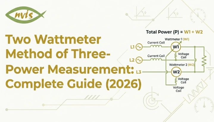
    Two Wattmeter Method of Three Phase Power Measurement: Complete Guide

    TL;DR

    • This guide is written for engineering students, freshers, and GATE, SSC JE, and RRB JE aspirants who need a clear, exam ready understanding of two wattmeter methods for measuring power in three phase circuits.
    • The two wattmeter method uses only two wattmeters, not three, to measure total power in a three phase system, regardless of whether load is balanced or unbalanced, star connected or delta connected.
    • two core relationships are P = W1 + W2 for total power, andφ = tan⁻¹√3(W1−W2)/(W1+W2) for power factor angle in a balanced load.
    • Wattmeter readings change character with power factor: both readings are equal at unity pf, one wattmeter reads zero at 0.5 lagging pf, and one wattmeter reads negative below 0.5 pf.
    • This method remains a core skill for testing, commissioning, protection, and instrumentation engineers in India’s power sector in 2026, and it is distinct from consumer smart metering rollout under RDSS, which measures energy for billing rather than power for engineering analysis.

    Also Read,

    The two wattmeter method is a standard technique used in electrical engineering to measure total power in a three phase, three wire system using only two wattmeters instead of three. Also referred to as 2 wattmeter method in many textbooks and lab manuals, it works for both balanced and unbalanced loads, and for both star and delta connected systems, which is why it remains one of most widely used measurement techniques in power system testing, laboratory experiments, and competitive exam syllabi across India. This guide builds concepts from the ground up. It starts with what a wattmeter actually measures, moves into how two wattmeters are connected in a three phase circuit, derives two wattmeter method formula step by step, and works through a complete numerical example. It then covers how wattmeter readings behave at different power factors, where method is applied in real power systems, its practical limitations, and how this classical method connects to digital instrumentation and smart metering landscape shaping India’s power sector in 2026. A dedicated section also maps out career paths and salary expectations for engineering students who build expertise in this area.

    What Is a Two Wattmeter Method?

    A wattmeter is an instrument that measures real power, also called active power, in an electrical circuit. It does this by combining two measurements at once: the current flowing through the circuit and the voltage across it. Internally, a wattmeter has two coils. The current coil is connected in series with the circuit, so the same current that flows through the load also flows through this coil. The pressure coil, also called the voltage coil, is connected in parallel across the circuit to sense voltage. A wattmeter’s needle or digital display indicates the product of these two quantities, adjusted for the phase angle between them, to show the actual power being consumed. The two wattmeter method is a standard technique used to measure the total active power in a three-phase, three-wire system using only two wattmeters instead of three. It works for both balanced and unbalanced loads, as well as for both star (Y) and delta (Δ) connected systems, making it one of the most widely used methods for three-phase power measurement in laboratories and industrial power systems.

    Why Three Phase Systems Need It?

    In a single-phase circuit, one wattmeter is enough because there is only one phase to measure. A three-phase circuit is more complex because it has three separate phases, and in principle, each phase requires its own power measurement. In a three-phase, four-wire system with an accessible neutral conductor, three wattmeters connected between each phase and the neutral can directly measure the total power. Most industrial and power distribution systems, however, are three-phase, three-wire systems without an accessible neutral. In such systems, Blondel’s theorem states that the total power can be measured using one fewer wattmeter than the number of wires. Since a three-wire system has three conductors, only two wattmeters are required to measure the total active power accurately. This is the fundamental principle behind the two wattmeter method, allowing it to measure total power correctly for both balanced and unbalanced three-phase loads.

    Two Wattmeter Method Circuit Connection

    The physical connection of two wattmeters follows a consistent rule regardless of whether load is star connected or delta connected. Current coils of two wattmeters are connected in series with any two or three line conductors, commonly labelled R and Y, or A and B, depending on the naming convention used. No current coil is connected to the third line, commonly labelled B or C. Pressure coils of both wattmeters are then connected between the line carrying their respective current coil and the third, unmeasured line. In other words, one wattmeter’s pressure coil spans between line R and line B, while the other spans between line Y and line B. This means both pressure coils share a common connection point on the third line, even though no current coil is placed there.

    Star (Y) Connected Load

    In a star connected system, the load’s three phases meet at a common neutral point, but this neutral point is typically not accessible or not used in a three wire supply. Two wattmeters are connected exactly as described above, with their current coils in two of three lines and their pressure coils referenced to the third line. The absence of a neutral connection does not affect the accuracy of the method, since two wattmeter methods are designed specifically to work without one.

    Delta (Δ) Connected Load

    In a delta connected system, there is no neutral point at all, since each phase winding connects directly between two line conductors. The two wattmeter method applies here in exactly the same way as it does for a star connected load, because the method depends only on three line conductors, not on how the load’s internal windings are arranged. This is one of the practical advantages of the method: the same two wattmeter connection setup works whether the underlying load is star or delta connected, and the engineer performing the test does not need to know the internal configuration in advance.

    Two Wattmeter Method Formula and Derivation

    Two wattmeter method formulas can be derived by analyzing a balanced three phase star connected inductive load. Consider a balanced system where phase voltage magnitude is V, line current magnitude is I, and load has a lagging power factor angle of φ between each phase voltage and its corresponding phase current. Each wattmeter measures the product of a line current, a line voltage, and cosine of angle between them. Using standard phasor analysis, current in wattmeter W1 lags its reference line voltage by an angle of (30° minus φ), while current in wattmeter W2 lags its reference line voltage by an angle of (30° plus φ). Since both wattmeters are referenced to line voltages of equal magnitude VL and carry line currents of equal magnitude IL in a balanced system, their individual readings work out to: W1 = VL IL cos(30° φ) W2 = VL IL cos(30° + φ) Adding these two expressions and simplifying using standard trigonometric identities produces a clean result. angle terms combine in such a way that sum equals: W1 + W2 = √3 VL IL cos φ This expression is exactly standard formula for total power in a balanced three phase system, confirming that sum of two wattmeter readings gives correct total active power, written as: P = W1 + W2 The individual readings can also be used to extract power factor angle without needing to measure it separately. Subtracting two wattmeter expressions and dividing by their sum removes the VL IL term and leaves only trigonometric functions of φ. Working through this algebra gives power factor angle formula: φ = tan⁻¹ [√3 (W1 W2) / (W1 + W2)] Once φ is known, the power factor itself is simply cos φ. This derivation assumes a lagging power factor and a balanced load. For an unbalanced load, sum W1 + W2 still gives correct total power, but power factor angle formula above does not apply, since power factor is only a meaningful single value for a balanced three phase load.

    Two Wattmeter Method Numerical Example

    A numerical example makes measurement of three phase power by two wattmeter methods easier to apply in practice. Consider a balanced three phase load connected to a 400 V line to line supply, drawing a total power of 10 kW at a lagging power factor of 0.8. The first step is to find the power factor angle. Since power factor is 0.8, φ = cos⁻¹(0.8), which works out to approximately 36.87°. The next step uses the power factor angle formula in reverse. Rearranging φ = tan⁻¹[√3(W1 W2)/(W1 + W2)] gives: tan φ = √3 (W1 − W2) / (W1 + W2) Since W1 + W2 = P = 10 kW, and tan(36.87°) is approximately 0.75, substituting these values gives: 0.75 = √3 (W1 W2) / 10 Solving this equation gives the difference between the wattmeter readings: W1 − W2 ≈ 4.33 kW. With two equations now available, W1 + W2 = 10 kW and W1 − W2 = 4.33 kW, solving simultaneously gives W1 = 7.165 kW and W2 = 2.835 kW. These two values represent what an engineer would actually observe on two wattmeter displays during a real test on this load. Adding them back together confirms total power of 10 kW, and the difference between them reflects the load’s lagging power factor of 0.8. This same step by step approach applies to any balanced three phase power measurement problem, and it is the method most frequently tested in GATE Electrical Engineering and SSC JE Electrical numerical questions.

    Wattmeter Readings at Different Power Factors

    The relationship between two wattmeter readings and the load’s power factor is not linear, and it produces several distinct patterns that are important to recognize, both for practical testing and for exam preparation. The table below summarizes how readings behave across the power factor range for a balanced lagging load.
    Power Factor Angle φ Wattmeter Behavior
    Unity (1.0) Both wattmeters read exactly equal values; each shows half total power.
    Above 0.5 lagging 0° to 60° Both wattmeters read positive, but unequal, values; W1 reads higher than W2.
    Exactly 0.5 lagging 60° One wattmeter (W2) reads exactly zero; the other reads full total power.
    Below 0.5 lagging 60° to 90° lower reading wattmeter (W2) becomes negative; its terminals must be reversed to obtain a reading, and this value is then subtracted rather than added.
    Zero (purely reactive) 90° Both wattmeters read equal and opposite values, and sum correctly shows zero real power.
    The case at 0.5 lagging power factor deserves particular attention, since it is one of most commonly tested scenarios. At this exact power factor, angle φ equals 60°, which makes angle term (30° minus φ) in wattmeter expression equal to negative 30°. Since cosine of negative 30° is a positive value, this wattmeter still reads a value, but companion expression works out so that one of two wattmeters reads exactly zero. This is not a fault or a wiring error; it is an expected mathematical outcome at that specific power factor. Below 0.5 lagging power factor, angle (30° plus φ) exceeds 90°, which makes its cosine negative. In practice, this means the pointer of an analog wattmeter would try to deflect backward, and standard procedure is to reverse connections of either current coil or pressure coil on that wattmeter to obtain a positive reading, then treat that reading as negative in calculation. Digital wattmeters typically display this as a negative value directly without requiring manual reversal. A separate limitation worth noting at this stage is that the two wattmeter method, by itself, cannot indicate whether the power factor is leading or lagging. The formula produces the same magnitude of φ for a leading load as it does for a lagging load with same wattmeter readings, since mathematics only reveals relative difference between readings, not direction of phase shift. In practice, engineers resolve this ambiguity by using auxiliary methods, such as briefly connecting a third reference wattmeter or using a known reactive element to determine load’s actual nature before or during test.

    Applications of the Two Wattmeter Method

    The two wattmeter method is widely used to measure total active power and power factor in three-phase, three-wire systems. Since it works for both balanced and unbalanced loads, it remains an important technique in electrical engineering. Some common applications include:
    • Testing and commissioning of transformers, motors, generators, and switchgear to verify power consumption against design specifications.
    • Protection and metering for calibrating protective relays, revenue meters, and other power measurement equipment.
    • Electrical engineering laboratories, where it is a standard experiment for studying three-phase power measurement and circuit analysis.
    • Motor testing, particularly for evaluating the power drawn by three-phase induction motors and synchronous machines under different operating conditions.
    • Renewable energy and EV charging systems, where similar measurement principles are used in digital instrumentation to verify power flow and power factor.
    It is important to distinguish this engineering method from India’s RDSS smart meter rollout. As of March 2026, 6.13 crore smart meters had been installed across the country under RDSS and other government and state schemes, with 4.69 crore installed under RDSS alone. These smart meters are designed for consumer energy metering and billing, whereas the two wattmeter method is used for engineering applications such as equipment testing, commissioning, protection, and instrumentation. Although modern digital power analyzers have largely replaced analog wattmeters, they continue to operate on the same fundamental principles as the two wattmeter method.

    Limitations and Practical Precautions

    While the two wattmeter method is accurate and widely used, a few practical limitations should be considered during testing.
    • Instrument transformer errors: Current transformers (CTs) and potential transformers (PTs) can introduce small phase-shift errors, especially at low power factors, affecting wattmeter accuracy.
    • Correct connections are essential: The current and pressure coils must be connected with the correct polarity. Incorrect connections can result in wrong or negative wattmeter readings.
    • Cannot identify leading or lagging power factor: The method calculates the magnitude of the power factor angle but cannot determine whether the load is leading or lagging without additional information.
    • Proper instrument ratings: Wattmeters and CTs should be rated for the expected line current and voltage to ensure accurate measurements and prevent instrument damage. Standard electrical safety practices should always be followed when working on live three-phase circuits.

    Future of the Two Wattmeter Method

    The classical electrodynamometer wattmeter, with its analog needle display, has largely been succeeded in modern testing environments by digital and microprocessor based power analyzers. Instruments in this category, produced by manufacturers such as Yokogawa and others, apply the same underlying two wattmeter mathematical principle internally, but they compute readings digitally rather than through a mechanical mechanism. These digital instruments offer several practical advantages, including automatic compensation for phase errors introduced by current and potential transformers, real time display of individual phase power alongside total power and power factor, harmonic analysis capability, and built in data logging with communication interfaces such as Modbus and Ethernet for integration into larger monitoring systems. This shift toward digital instrumentation does not change underlying physics or mathematics covered in this guide. Whether an engineer is reading an analog wattmeter dial in a college laboratory or interpreting a digital display on a modern power analyzer during a substation commissioning test, two wattmeter principles, formula P = W1 + W2, and power factor relationship derived from two readings remain exactly the same. Understanding classical methods thoroughly is what allows an engineer to correctly interpret, troubleshoot, and validate output of any modern digital instrument built on the same foundation. At same time, India’s power sector is undergoing significant modernization on the metering side, driven by RDSS smart meter rollout and CEA’s 2026 regulatory push toward mandatory smart metering for consumers. This transformation is reshaping how electricity is billed and monitored at consumer level, but it operates alongside, rather than in place of, engineering side power measurement skills covered in this guide. For students entering the workforce, familiarity with both classical two wattmeter methods and digital instrumentation that has grown from it provides a stronger technical foundation for roles across testing, commissioning, protection, and instrumentation engineering.

    Conclusion

    The two wattmeter method remains one of the most fundamental techniques in three phase power measurement, valued for its ability to determine total active power and power factor in balanced or unbalanced, star or delta connected loads using just two instruments instead of three. Its derivation rests on straightforward phasor analysis, its formula P = W1 + W2 is simple to apply once underlying connection is understood, and its special case behavior at different power factors, including zero reading case at 0.5 lagging pf and negative reading case below it, follows predictable and learnable patterns rather than being arbitrary exceptions. For engineering students in India, mastering this method serves a dual purpose: it builds conceptual foundations tested repeatedly in GATE, SSC JE, and RRB JE examinations, and it develops a practical skill directly applicable to testing, commissioning, protection, and instrumentation roles across the power sector. As India’s power infrastructure continues to modernize through initiatives such as RDSS smart meter rollout and evolving CEA regulations, underlying measurement principle behind two wattmeter method continues to operate quietly within digital power analyzers now used across industry, making it a technique worth understanding thoroughly rather than memorizing for a single exam.

    FAQs

    The two wattmeter method is a technique used in electrical engineering to measure total active power in a three phase, three wire system using only two wattmeters. It works for both balanced and unbalanced loads and for both star and delta connected systems, with total power given by sum of two wattmeter readings.

    The two -wattmeter method formula for total power is P = W1 + W2. For a balanced load, power factor angle can be calculated using φ = tan⁻¹√3(W1−W2)/(W1+W2) after which power factor itself is obtained as cos φ.

    The sum of two wattmeter readings gives correct total power regardless of whether load is balanced or unbalanced. power factor angle formula, however, applies only to balanced loads, since power factor is not a single defined value for an unbalanced three phase load.

    The formula used to calculate power factor angle produces the same magnitude of φ whether load is leading or lagging, since it depends only on the difference between two wattmeter readings rather than direction of phase shift. Determining whether power factor is leading or lagging requires additional information about load or an auxiliary measurement.

    At exactly 0.5 lagging power factor, one of two wattmeters reads exactly zero while the other reads full total power. Below 0.5 lagging power factor, lower reading wattmeter reads a negative value, which must be subtracted rather than added when calculating total power.

    Yes. India’s RDSS smart meter rollout and CEA’s 2026 metering regulations concern consumer energy billing, which is a separate function from engineering power measurement. The two -watt meter method remains the underlying principle used in testing, commissioning, protection calibration, and even in digital power analyzers that have replaced older analog wattmeters in modern power system work.

    What Is a De Sauty bridge? Working Principle & Experiment

    TL;DR

    • This blog is for engineering students, electronics lab freshers, and anyone meeting bridge circuits for the first time, explaining De Sauty bridge in plain language before formulas show up.
    • A De Sauty bridge is a simple AC circuit used to compare an unknown capacitor against a known one, using a point where a headphone or detector goes silent as “answer.”
    • The core idea is balance, not complicated math. Once you understand why zero current in the detector arm means something useful, the whole circuit clicks.
    • De Sauty bridge experiment follows a repeatable procedure: set up four arms, apply an AC signal, adjust a resistor until you hit a null point, then calculate unknown capacitance from a simple ratio.
    • The bridge has one real weakness, dielectric loss in real world capacitors, and Grover’s modification exists specifically to fix it. Understanding that limitation is often exact thing exam questions test.

    Also read,

    Desauty bridge is a foundational AC bridge circuit used in electrical measurement to compare an unknown capacitor against a known standard capacitor. It remains a core part of electrical and electronics engineering lab curricula across Indian universities, both as a practical measurement method and as an introduction to balance principle used throughout instrumentation.

    This guide explains how De Sauty bridge works, breaks down circuit and its components, and walks through De Sauty bridge experiment step by step, including observation table, calculation method, and common troubleshooting points. It also covers bridge’s key limitation with real capacitors, modifications introduced to address it, and where the same balancing principle continues to appear in current engineering research.

    What Is a De Sauty bridge?

    A De Sauty bridge is an AC bridge circuit used to measure or compare capacitance. In simple terms, it is a tool that tells you the value of an unknown capacitor by comparing it against a capacitor whose value you already know. It was developed by French engineer Paul de Sauty as one of earliest reliable methods for capacitor comparison, and it still shows up in electrical measurement labs across Indian engineering colleges today. The reason it has survived this long is simple: the circuit is easy to build, the math behind it is straightforward, and it teaches a concept that shows up everywhere in instrumentation, idea of balance.

    Unlike a multimeter or a modern LCR meter that gives you a direct digital reading, a De Sauty bridge works by comparison. You adjust the circuit until it reaches a specific balanced state, and at that exact point, a simple ratio tells you unknown capacitance. It sounds old fashioned, and in some ways it is, but the underlying principle is the same one used inside far more advanced capacitance sensing systems today.

    How a Bridge Circuit Actually Balances?

    Before touching De Sauty bridge specifically, it helps to understand what a “bridge circuit” even means, because the word confuses a lot of first time learners.

    Think of a bridge circuit as two parallel paths carrying the same electrical signal from a source to a detector. If both paths are perfectly matched, no difference in voltage appears between them, and a detector connected across the middle of two paths sees nothing, no current, no signal, no deflection. That state is called balance.

    If two paths are not matched, there is a small voltage difference between them, and the detector picks it up. In older lab setups, that detector is often a pair of headphones connected through a small transformer, and instead of a needle moving, you literally hear a tone. As you adjust a resistor toward the correct value, tone gets quieter. At the exact balance point, sound disappears completely. That silent moment is called null deflection, and it is the entire trick behind how a De Sauty bridge works.

    This matters because once you understand that balance simply means “both paths are now electrically identical,” the rest of the circuit stops feeling like memorized formulas and starts feeling like basic logic.

    De Sauty bridge Circuit Diagram and Components

    A De Sauty bridge has four arms arranged in a diamond or square shape, with an AC source connected across one diagonal and a detector connected across other diagonals.

    Here is what typically sits in each arm:

    Arm 1, contains an unknown capacitor, one whose value you are trying to find. Arm 2, contains a standard, known capacitor used as reference. Arm 3 and Arm 4, contain two non inductive resistors, meaning resistors built specifically so they do not behave like tiny inductors at AC frequencies. This matters because any stray inductance would throw off the balance condition.

    An AC signal, usually from an audio oscillator around 1 kHz, is applied across one pair of opposite corners of this diamond. A detector, either a headphone based null detector or a digital null indicator in more modern trainer kits, is connected across other pairs of corners.

    The basic idea is this: current splits and flows through both halves of the bridge at once, one half containing unknown capacitor and one resistor, the other half containing standard capacitor and other resistor. When the ratio of components on both sides matches perfectly, the detector arm carries zero current, and you have found your balance point.

    De Sauty bridge Working Principle

    Once physical layout makes sense, the working principle becomes much easier to follow.

    De Sauty bridge works on principle of null deflection, which just means the circuit is adjusted until the detector shows no response at all. In an AC circuit, “no response” happens when electrical opposition, called impedance, on both halves of the bridge becomes proportionally equal. Impedance in this context is essentially resistance and capacitive effects combined, since capacitors do not behave like plain resistors under AC signals.

    Balance Condition and Capacitance Formula

    At balance, the impedance ratio across two arms is equal, which for this bridge simplifies into a very clean relationship between two capacitors and two resistors. Written simply, unknown capacitance equals standard capacitance multiplied by ratio of two resistor values.

    Usually labeled R1 or R3 depending on the kit, balance condition gives:

    C1 = C2 × (R4 / R3)

    This is genuinely one of simplest formulas in electrical measurement, and that simplicity is exactly why De Sauty bridge is often the first bridge circuit taught to engineering students before more complex bridges like Maxwell’s or Schering’s bridge. You are not just learning one formula, you are learning a logic pattern that every other bridge circuit in your syllabus will reuse.

    De Sauty bridge Experiment: Step by Step Procedure

    This is part most lab manuals rush through, so here is the De Sauty bridge experiment broken down clearly, way it is typically performed on a standard trainer kit in a college lab.

    Objective: To determine unknown capacitance of a capacitor using a De Sauty bridge.

    Apparatus required: A De Sauty bridge trainer kit (with built in decade resistance dials and a standard capacitor), an audio frequency oscillator, a headphone or digital null detector, connecting wires, and unknown capacitor to be tested.

    Procedure:

    First, connect an unknown capacitor to the terminal marked for it on the trainer board. Next, connect the audio oscillator across the excitation terminals of the bridge, and connect the headphone or null detector across the detector terminals.

    Switch on the oscillator. At this stage, you should hear a tone through headphones, or see a live reading on a digital null detector, confirming the bridge is receiving a signal but is not yet balanced.

    Now slowly vary the resistance dial, usually labeled R1 or R3 depending on the kit, while listening carefully to headphone output, or watching detector reading. As you approach balance, tone will noticeably reduce in volume, or detector reading will drop toward zero.

    Adjust carefully around this point until sound disappears entirely, or the detector shows minimum deflection. This is your null point. Note down resistance values at this exact setting.

    Repeat this process at least three to five times, either by slightly disturbing and re-finding the balance point, or by testing with a different known standard capacitor value, to reduce impact of small human or instrument error.

    Why De Sauty bridge Struggles with Real Capacitors

    De Sauty bridge assumes every capacitor in circuit is a “pure” or ideal capacitor, one that only stores and releases energy without wasting any of it as heat.

    Real capacitors are not perfectly ideal. Every practical capacitor has some internal energy loss caused by insulating material between its plates, called dielectric. This loss is known as dielectric loss, and it behaves almost like a hidden resistor sitting inside a capacitor.

    Because the standard De Sauty bridge formula only accounts for pure capacitance and pure resistance, it cannot properly balance, or gives an inaccurate reading, when dielectric loss is significant. This is the single biggest limitation of basic De Sauty bridge, and it is almost guaranteed to come up as a viva question in your practical exam.

    Grover’s Modified De Sauty bridge

    To fix this dielectric loss problem, a modification was introduced, commonly credited to Grover, which adds two extra resistors into arms containing capacitors themselves.

    These additional resistors are specifically placed to represent and account for internal loss inside each capacitor. With this change, a modified bridge can accurately measure both capacitance value and dissipation factor, a number that represents how “lossy” or imperfect a real capacitor actually is.

    In practical terms, this modification turns De Sauty bridge from a circuit that only works on textbook perfect capacitors into one that can meaningfully test real components, which is exactly why modified versions appear in more advanced instrumentation labs and even in some published engineering research today.

    Where De Sauty bridge Principle Shows Up Today

    It is easy to assume a circuit this old is purely academic, something you learn for an exam and then forget. That is not entirely true.

    The core balancing principle behind De Sauty bridge is still actively used in modern capacitive sensing research. Engineers working on structural health monitoring, practice of using sensors to detect tiny stress cracks or strain in bridges, buildings, and aircraft structures, have built wireless capacitive strain sensors around an analog De Sauty bridge design, precisely because balance based approach is sensitive enough to detect extremely small capacitance changes. Similar autobalancing versions of De Sauty bridge have also been explored for wide range capacitive sensor interfaces in wearable and biomedical devices, including experimental sensors designed to track tremor related signals.

    This matters for you as a student because it reframes the entire lab experiment. You are not just learning a historical measurement trick, you are learning the exact same balance principle that underpins how many present day capacitive sensors are designed and calibrated. commercial LCR meters and digital bridge instruments used in modern electronics testing trace their conceptual roots directly back to bridge circuits like this one.

    Advantages and Disadvantages of De Sauty bridge

    De Sauty bridge earns its place in every basic electrical measurements syllabus for a few clear reasons, but it also comes with limitations worth knowing before your practical exam.

    Advantages: circuit design is simple and inexpensive to build. The balance formula is easy to derive and calculate by hand. It offers good accuracy when measuring capacitors that are close to ideal, and it is an excellent teaching tool because it introduces the null deflection concept used throughout electrical instrumentation.

    Disadvantages: basic version cannot accurately measure capacitors with meaningful dielectric loss, which covers a large share of real world capacitors. It requires a stable AC source and a sensitive detector to find a clean null point, and manually adjusting resistors to reach balance is slower than simply reading a value off a digital LCR meter.

    Conclusion

    De Sauty bridge is one of those rare topics that looks intimidating on paper but makes complete sense once you understand the single idea driving it, balance. Four arms, an AC signal, a detector listening for silence, and one clean formula connecting an unknown capacitor to a known one. That is the entire circuit, stripped of textbook language.

    Running the De Sauty bridge experiment yourself is the fastest way to make this concept permanent rather than something memorized the night before an exam. Once you have physically turned that resistance dial, heard tone fade into silence, and calculated your first unknown capacitance from real observation data, bridge circuits as a whole, including more advanced ones waiting later in your syllabus, stop feeling like a wall of formulas and start feeling like a pattern you already understand. If you are heading into your electrical measurements lab this semester, keep this guide open beside your manual, and if a topic still feels unclear after your first attempt at experiment, that usually means it is worth revisiting once more before viva day rather than after.

    FAQs

    A De Sauty bridge is mainly used to measure or compare the value of an unknown capacitor against a known standard capacitor. It is a foundational instrument taught in electrical and electronics measurement labs to introduce the concept of AC bridge balancing.

    Headphones are used because they are extremely sensitive to small AC signals at audio frequencies, making it easy for a student to hear the exact moment the bridge reaches null deflection. Some modern trainer kits replace headphones with a digital null detector for the same purpose.

    At balance, unknown capacitance C1 equals standard capacitance C2 multiplied by the ratio of two resistors, written as C1 = C2 × (R4 / R3). This formula is derived directly from the impedance balance condition of the bridge.

    The basic De Sauty bridge assumes capacitors are ideal and lossless, but real capacitors have internal dielectric loss. This loss is not accounted for in the standard formula, which is why the bridge gives unreliable readings for capacitors with significant loss, unless a modified version is used.

    Grover’s modification adds extra resistors into capacitor arms of the bridge specifically to account for dielectric loss. This allows modified De Sauty bridge to accurately measure both capacitance and dissipation factor of real, imperfect capacitors.

    Yes. While digital LCR meters have replaced it for routine industrial measurement, the underlying balance principle of De Sauty bridge is still used in current research areas like wireless structural health monitoring sensors and wide range capacitive sensor interfaces, making it more than just a historical lab exercise.

    Tags: De Sauty bridge

    Request a Callback

    Please enable JavaScript in your browser to complete this form.

    No spam. Just a quick call.

    =