8051 Microcontroller: Architecture, Working, Pins and Applications

Posted on 27-08-202628-08-2026 by Tushar Saluja

TL;DR

This blog is for engineering freshers, university students, and GATE/SSC JE/RRB JE aspirants who want to understand 8051 microcontroller architecture from ground up, without getting lost in jargon.
8051 microcontroller packs a CPU, memory, timers, I/O ports, and a serial port onto a single chip, which is why it remains a commonly used teaching platform for learning embedded-system fundamentals in India.
This blog breaks down internal architecture, 40-pin layout, and how 8051 actually processes instructions, using plain language and a worked numerical example.
You will also see where 8051 fits into Indian engineering education, legacy industrial systems, automotive applications, and consumer electronics, along with its relevance to exams and embedded-systems careers.
By the end, you will be able to explain 8051 architecture confidently in interviews, labs, and competitive exams like GATE, SSC JE, and RRB JE.

The 8051 is an 8-bit microcontroller originally introduced by Intel in 1980. It uses a modified Harvard architecture, with separate program and data memory spaces. 8051-compatible devices are still offered by several semiconductor manufacturers. It integrates a CPU, RAM, ROM, I/O ports, timers, and a serial communication port on a single chip, which is what separates a microcontroller from a microprocessor. This guide explains 8051 microcontroller architecture section by section, walks through its 40-pin configuration, and connects each concept to real applications and exam preparation for Indian engineering students.

What Is 8051 Microcontroller, and Why Does It Matter?

Consider a remote control for ceiling fans. Fans automatically adjust speed by simply pressing a button. There is no separate processor chip, no separate memory chip and no separate circuit to sense when you press the button inside that remote. It all resides on a single chip. The chip is a microcontroller.

In essence, a microcontroller is a very small computer that fits into one silicon chip. It is composed of a processor that performs thinking, memory that stores instructions and data, and input-output pins to communicate with the outside world such as buttons, motors, and displays. A traditional microprocessor typically relies on external memory and peripheral components, whereas a microcontroller integrates a processor, memory, and peripherals on a single chip. A microcontroller has all that built-in, making it cheaper, smaller and easier to design with.

The 8051 became a popular teaching platform because its relatively simple architecture makes concepts such as registers, timers, interrupts, I/O, and memory organization easier to demonstrate. Many Indian engineering programmes continue to use the 8051 to introduce students to microcontroller fundamentals before moving to newer platforms such as STM32 and ESP32. If you can describe how the 8051 fetches, decodes, and executes an instruction, you will understand the basic instruction-execution concepts that apply across many processors and microcontrollers.

8051 Microcontroller Architecture: Big Picture

Think of a small office with one manager (CPU) with a personal notepad (registers), a filing cabinet (RAM) in which to keep the daily paperwork, a locked archive (ROM) in which to keep the instructions to be used for the rest of the manager’s life, and telephone lines (I/O ports and serial port) for communicating with the outside world. All of the manager’s responsibilities can be accomplished in that one office. The architecture of the 8051 microcontroller is precisely like that.

The heart of the 8051 microcontroller architecture is an 8-bit CPU, meaning that it works with 8 bits (1 byte) of data. The classic 8051 uses an 8-bit data path and a 16-bit address space for program and external data memory. Because the 8051 uses separate 16-bit address spaces for program memory and external data memory, each address space can theoretically cover up to 64 KB. The 8051 uses 16-bit addressing for its program and external data memory spaces, allowing each space to address up to 64 KB.

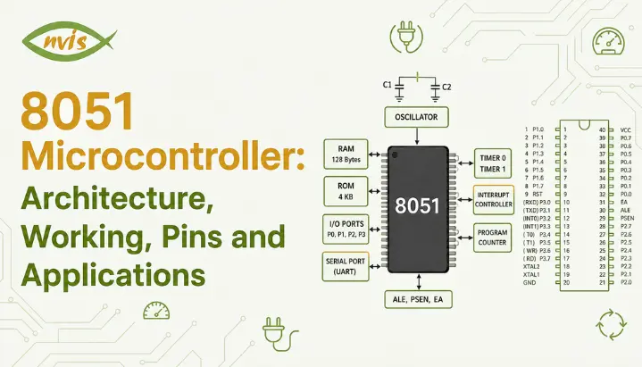
major building blocks of architecture of 8051 microcontroller are:

The CPU is the “brain” and retrieves instructions from memory, decodes their meaning and carries them out sequentially. The CPU contains Arithmetic Logic Unit (ALU) that carries out addition/subtraction and logical comparisons, accumulator (ACC) – a special register that stores the outcome of most operations.

memory is divided into two distinct memory spaces, program memory and data memory, This separation of program and data memory spaces is a defining characteristic of the 8051’s modified Harvard architecture. In contrast, a conventional Von Neumann architecture uses a shared memory space for instructions and data. In the original 8051, the on-chip program memory is 4 KB of ROM, while the internal RAM is 128 bytes. Program memory stores the program code, while RAM stores temporary data used during execution.

The chip can read switches, sensors, and buttons through four, 8-bit-wide I/O ports (P0, P1, P2, P3) and control LEDs, motors, and displays.

timers and counters, two of which are 16 bits, provide accurate time delays and counting of external events which are critical for many timing operations, such as flashing an LED at a specific time interval or counting the speed of a motor.

The 8051 has a full-duplex serial port that can transmit and receive data serially. Its TXD and RXD lines are available on P3.1 and P3.0 respectively, and the serial interface supports UART-style communication.

An interrupt system will allow the microcontroller to stop what it’s doing and react to some very urgent process, such as a button being pressed, without having to continuously scan for the event in a loop.

CPU: Decision-Making Core

Imagine a calculator that has a memory for the function just performed and that can determine what to do next based on the results of that function. It’s basically the 8051 CPU. It has ALU for arithmetic and logic operations, accumulator (register A), a special register named B that is used during multiply and divide operations, a group of general purpose registers (R0 to R7) used as temporary scratch pads.

CPU also has a special register called a Program Status Word (PSW) that contains bits that can be used as dashboard status lights. It contains status flags such as Carry (CY), Auxiliary Carry (AC), and Overflow (OV), along with register-bank selection bits and the parity flag. The classic 8051 PSW does not have a dedicated zero flag. These flags are continually scanned by a programmer to determine its value and thereby make a decision, just as you look at the fuel light in your car before you stop for petrol.

Memory Organization: Two Separate Filing Systems

This is a very practical analogy with which to work. Program memory is like a recipe book because it stores the instructions the CPU follows. Data memory is like a kitchen counter because it temporarily holds the data and values being worked on. The recipe book represents program memory because it stores the instructions the CPU follows, while the kitchen counter represents RAM, where temporary data can be read and changed during execution. Ingredients are placed on the kitchen counter and you can mix things and constantly update on what’s happening in the kitchen. With 8051, the ROM was like a recipe book, and the RAM was like a kitchen counter.

The original 8051 has 4 KB of on-chip program ROM and 128 bytes of internal RAM. It can also address up to 64 KB of external program memory and up to 64 KB of external data memory. Program ROM retains the stored program even when power is removed, which is why it is classified as non-volatile memory.

Data memory (RAM) is 128 bytes. The lower 32 bytes contain four register banks, the next 16 bytes are bit-addressable, and the remaining 80 bytes are general-purpose RAM. Special Function Registers (SFRs) are located in a separate address space from this 128-byte internal RAM.

The 8051 uses separate program and data memory spaces, allowing code and data to be addressed independently. This separation is a key characteristic of its modified Harvard architecture.

Worked Example: Suppose you want to know how many distinct memory locations 8051’s 16-bit address bus can access. A 16-bit address bus can represent 2^16 combinations, since each bit can be either 0 or 1.

2^16 = 65,536 locations, which equals 64 KB.

This is why you will often see “64 KB program memory” and “64 KB external data memory” mentioned in 8051 datasheets. 16-bit address bus is physical reason behind that 64 KB limit, and this exact kind of calculation shows up regularly in GATE and PSU written exams when they ask you to compute addressable memory from bus width.

Timers and Counters: Keeping Time Without a Wristwatch

Suppose you want the LED to turn on and off precisely once every second, without having to count seconds. There’s a component in the chip that can reliably count clock pulses, but your main program is doing other work, i.e. you want a clock to count in the background. That’s the job of Timer 0 and Timer 1.

Each timer uses a 16-bit counting register. In timer mode, it increments based on the internal machine-cycle timing; in counter mode, it increments in response to external transitions applied to its counter input, such as counting the number of times the conveyor belt sensor is triggered. When the timer is filled to its maximum value and wraps around to zero again, it may interrupt your program and indicate that a fixed period of time has elapsed.

The timers are configured and controlled using the 8-bit TMOD (Timer Mode) and TCON (Timer Control) registers. The timer modes determine whether the timer operates as a 13-bit timer, 16-bit timer/counter, 8-bit auto-reload timer, or, for Timer 0, two separate 8-bit timers.

I/O Ports: Chip’s Hands and Ears

The only real connection between 8051 and the physical world is the 8 pins per port (P0, P1, P2, P3) for a total of 32 general purpose I/O lines.

Port 0 is special as it serves double purpose. In designs that do not use external memory, Port 0 can be used as a general-purpose bidirectional I/O port, but it requires external pull-up resistors because it does not have internal pull-ups in the classic 8051. In larger designs, in which external memory is connected, Port 0 carries a lower byte of address and data, multiplexed onto the same pins; this is a smart use of pin space on the chip.

Most variants of the 8051 do not have an alternative function for port 1, making it the easiest port to use for simple input/output (I/O) applications, such as attaching LEDs and switches.

Port 2 can be used as general-purpose I/O or, when external memory is accessed, it carries the higher-order address byte (A8–A15).

The port 3 has multiple alternate functions that are vital to the operation of the chip, such as serial port’s transmit and receive lines, two external interrupt inputs, and the external count input for the timer.

Pin Diagram and Pin Description of 8051 Microcontroller

The 8051 microcontroller is packaged as a 40-pin Dual Inline Package (DIP), and understanding what every pin does is what actually lets you wire a circuit or answer a pin-diagram question correctly in an exam. Here is a pin-by-pin breakdown.

Pins 1 to 8 form Port 1 (P1.0 to P1.7), a general-purpose bidirectional I/O port with no alternate functions in base 8051, making it the simplest port to use for connecting external devices like LEDs or push buttons.

Pin 9 is RST, Reset pin. Applying a HIGH level to the RST pin for at least two machine cycles while the oscillator is running resets the microcontroller and places its registers and control logic into their defined reset states, similar to restarting your computer when it freezes.

Pins 10 to 17 form Port 3 (P3.0 to P3.7), which carries important alternate functions: P3.0 (RXD) and P3.1 (TXD) handle serial communication, P3.2 (INT0) and P3.3 (INT1) are external interrupt inputs, P3.4 (T0) and P3.5 (T1) are external timer/counter inputs, and P3.6 (WR) and P3.7 (RD) control write and read operations to external memory.

Pin 18 and Pin 19 (XTAL2 and XTAL1) connect to an external crystal oscillator, which generates clock pulses that drive every internal operation, similar to a heartbeat that keeps the whole chip synchronized.

Pin 20 is GND, ground reference for the entire chip.

Pins 21 to 28 form Port 2 (P2.0 to P2.7), used as general I/O, or as higher-order address byte (A8 to A15) when external memory is connected.

Pin 29 is PSEN (Program Store Enable), an output pin that goes active-low specifically when the CPU reads from external program memory.

Pin 30 is ALE (Address Latch Enable), used to separate multiplexed address and data signals on Port 0 during external memory access.

Pin 31 is EA (External Access), which decides whether CPU executes code from internal ROM or external memory. For the classic 8051, EA determines whether program execution uses the internal program ROM or external program memory. With EA high, the device uses its internal program memory for the internal address range; with EA low, it fetches program code from external memory

Pins 32 to 39 form Port 0 (P0.0 to P0.7), used as general I/O in small designs, or as multiplexed lower-order address and data bus (AD0 to AD7) in designs with external memory. Port 0 has no internal pull-up resistors, so external pull-ups are needed if you want to use it as a plain output port.

Pin 40 is VCC, supplying +5V power that runs the entire chip.

How 8051 Microcontroller Works: Instruction Execution Cycle

Think about how you follow a recipe. You read one line, understand what it is asking you to do, then actually do it, before moving to the next line. 8051 does exactly this with program instructions, in a loop called fetch-decode-execute cycle.

First, the CPU fetches an instruction from program memory (ROM), using Program Counter (PC), a register that always points to the address of the next instruction to be read. Second, the CPU decodes that instruction, figuring out what operation it represents, whether it is an addition, a data move, or a jump to another part of the program. Third, CPU executes instruction, actually performing operation, which might update the accumulator, change a flag in PSW, or toggle an I/O pin.

This entire cycle repeats continuously, driven by clock signals from external crystal oscillators connected at pins 18 and 19. The classic 8051 uses 12 oscillator periods per machine cycle. Therefore, with a 12 MHz oscillator, one machine cycle takes 1 μs, although individual instructions may require one or more machine cycles, though exact instruction execution time varies depending on how many machine cycles that particular instruction needs.

8051 vs 8052 vs 8031: Knowing Family

Students often get confused between these three names, so here is a plain difference. 8051 is the standard version with 4 KB of internal ROM and 128 bytes of RAM. 8052 is an upgraded version with double ROM (8 KB), double RAM (256 bytes), and an additional third timer, making it useful for slightly more demanding applications. 8031 is essentially an 8051-family device without on-chip program ROM, so it requires external program memory.

Feature	8051	8052	8031
Internal ROM	4 KB	8 KB	None (external only)
Internal RAM	128 bytes	256 bytes	128 bytes
Timers	2 (16-bit)	3 (16-bit)	2 (16-bit)
Interrupt sources	5	6	5
Typical use case	General teaching and small embedded designs	Slightly larger programs needing more memory	Designs already using external memory

Where 8051 Microcontroller Is Used in India

Even with modern 32-bit microcontrollers dominating new product designs, 8051 continues to have a real footprint in Indian industry and education, mainly because so much existing equipment, teaching infrastructure, and legacy code still runs on it.

Historically, 8051-based controllers have been used in simple industrial control applications such as relay control, instrumentation, and small automation systems. Today, newer microcontrollers are generally preferred for new industrial designs, while knowledge of 8051 can still be useful when working with legacy equipment and older control systems. Legacy 8051-based control boards can still be relevant when engineers maintain or troubleshoot older industrial equipment, although specific implementations vary by plant and system, and understanding this architecture helps engineers troubleshoot and maintain that equipment.

In consumer electronics, appliances like washing machines, microwave ovens, and remote controls historically ran on 8051 variants, and 8051-class devices can still be suitable for some simple, cost-sensitive embedded applications, although the specific microcontroller chosen depends on the product’s requirements and design constraints.

In automotive systems, 8051-family devices have been used historically in automotive and vehicle-related embedded applications, particularly in simpler control and instrumentation systems.Modern automotive designs generally rely on more capable automotive-grade microcontrollers and processors. ARM-based microcontrollers and software platforms such as AUTOSAR are widely used in modern automotive development, particularly as vehicle electronics become more complex.

In defense and aerospace, older microcontroller-based systems may use architectures such as the 8051, but newer systems generally use processors and microcontrollers selected according to their performance, reliability, radiation tolerance, and system requirements.

In engineering education, Many Indian engineering programs have historically used 8051 as an introductory platform for teaching microcontroller fundamentals, because its instruction set is simple enough to teach in a semester while still covering every core microcontroller concept students need before moving to ARM-based designs.

Exam Relevance: GATE, SSC JE, and RRB JE

If you are preparing for competitive exams, here is exactly where 8051 microcontroller fits into your syllabus. For GATE EC, the 2026 syllabus does not list 8051 as a dedicated topic. Students should therefore focus on broader concepts such as machine instructions, addressing modes, ALU, datapath and control unit, along with relevant embedded-systems fundamentals. Therefore, students should focus on the underlying concepts rather than treating 8051-specific memorization as a separate GATE syllabus area. The current GATE 2026 EC syllabus should be used as the reference when discussing exam relevance. Therefore, 8051-specific memorisation should not be treated as a separate GATE EC preparation area. Instead, focus on the broader computer-organisation and digital-electronics concepts covered by the official syllabus.

For SSC JE and RRB JE preparation, 8051-related concepts may be relevant depending on the applicable syllabus and recruitment notification. Students should check the latest official syllabus before treating 8051 as a guaranteed topic. Depending on the recruitment notification and syllabus, questions may cover topics such as microcontroller architecture, pin functions, timers, interrupts, and addressing modes. Expect questions asking you to identify pin functions, calculate timer overflow values, or explain differences between Harvard and Von Neumann architecture using 8051 as a reference example.

In technical recruitment exams and interviews for electronics and embedded-systems roles, questions on 8051 fundamentals may be useful for assessing concepts such as timers, interrupts, memory organisation, and I/O such as architecture, timers, interrupts, and memory organization, since these fundamentals demonstrate whether a candidate genuinely understands embedded systems or has only memorized definitions.

Career and Salary Relevance for Embedded Systems Roles in India

Learning 8051 architecture can provide a useful foundation in embedded-systems concepts, especially for students and beginners, even though most production work today happens on more advanced 32-bit microcontrollers.

Freshers entering embedded systems roles in India can see a wide range of starting compensation depending on location, company, skills, internships, and role requirements, with exact figures depending on internships, hands-on project experience, and whether the candidate has exposure to modern platforms alongside fundamentals like 8051. Candidates who pair 8051-level architectural understanding with practical skills on platforms like STM32, AVR, or ESP32 tend to command the higher end of that range, since companies want engineers who understand fundamentals but can also work on current hardware.

Mid-level embedded engineers with three to five years of experience in India typically earn higher salaries than freshers, with compensation varying significantly by experience, location, company, and technical specialization. Senior embedded engineers and architects at major semiconductor and automotive companies can earn substantially more. Demand driving this growth includes India’s semiconductor manufacturing push under PLI scheme, expanding EV sector, and growing IoT adoption across industrial and consumer products.

For freshers, practical takeaway is this: learning 8051 microcontroller architecture thoroughly builds conceptual foundation, including memory organization, interrupts, timers, and register-level programming, that transfers directly to every other microcontroller you will work with in your career, from AVR to ARM Cortex-M.

Conclusion

8051 microcontroller architecture might be decades old, but it remains a clear and useful way to understand how many fundamental microcontroller concepts work, from CPU and memory organization to timers, I/O ports, and the instruction-execution cycle used by processors and microcontrollers. You now know how its 40 pins are organized, how its Harvard architecture separates program and data memory, and where this chip still shows up in Indian industry, exams, and interviews today.

The best next step is hands-on practice. Pick up an 8051 development board, write a simple LED-blinking program using Timer 0, and watch concepts from this blog come alive on actual hardware. If you are preparing for SSC JE, RRB JE, or a PSU interview, revisit pin diagrams and timer sections until you can redraw and explain them without looking back at your notes.

FAQs

What is the 8051 microcontroller used for?

The 8051 microcontroller is used in embedded systems that need to control hardware directly, including industrial automation panels, consumer appliances, basic automotive dashboard controls, and countless college and hobbyist projects. Its simplicity makes it ideal for learning core microcontroller concepts before moving to advanced platforms.

What is the architecture of the 8051 microcontroller based on?

The architecture of the 8051 microcontroller is based on a modified Harvard architecture, meaning program memory and data memory occupy separate address spaces, which is a defining characteristic of the 8051’s modified Harvard architecture.

How many pins does an 8051 microcontroller have, and what are they used for?

The 8051 microcontroller has 40 pins in its standard DIP package. Of these, 32 pins form four 8-bit I/O ports (P0 to P3), while remaining 8 pins handle power supply, ground, reset, crystal oscillator connections, and control signals for external memory access.

Is 8051 microcontroller still relevant in 2026?

Yes, though mainly for education, legacy system maintenance, and cost-sensitive consumer products rather than new high-performance product design. Many new embedded projects use more capable 32-bit microcontrollers and SoCs, including STM32-family devices and ESP32-family chips, but 8051 architecture remains a commonly used teaching example for introducing microcontroller fundamentals because it clearly demonstrates core concepts every embedded engineer needs.

What is the difference between a microprocessor and an 8051 microcontroller?

A microprocessor, like ones in laptops, only contains CPU and needs external chips for RAM, ROM, and I/O. 8051 microcontroller integrates CPU, RAM, ROM, I/O ports, timers, and a serial port all on a single chip, making it self-sufficient for embedded applications without needing external support circuitry.

How many timers does an 8051 microcontroller have?

standard 8051 has two 16-bit timers, Timer 0 and Timer 1, used for generating precise time delays or counting external events. upgraded 8052 variant adds a third timer, useful for applications needing an additional independent timing source.

STM32 Microcontroller Guide: How It Works, Programming, and Applications

Posted on 27-08-202627-08-2026 by Tushar Saluja

TL;DR

This blog is for engineering students, freshers, and first-time embedded learners in India who want to learn about STM32 microcontrollers from scratch without prior experience in microcontroller programming.
STM32 is a range of 32 bit microcontroller chips from STMicroelectronics based on ARM Cortex M processor cores, and is one of the world’s most widely used 32bit microcontroller families.
This guide is designed to explain the STM32 uses and family of chips (STM32F, STM32L, STM32H, STM32G, STM32WB, STM32WL series), as well as how to program an STM32 using STM32CubeIDE, and finally has two worked numerical examples included for exam preparation.
It also elaborates on the context of India embedded technology based on STM32 used in the Indian industry, relevance of GATE & PSU exams and realistic salary expectations for embedded freshers.
At the end of this, you will be able to select a board, configure STM32CubeIDE and see what is now happening in the chip when the code is executed.

STM32 is a range of 32 bit microcontroller chips from STMicroelectronics based on ARM Cortex M processor cores. It is one of the most popular microcontroller platforms in use today in embedded systems applications ranging from the student robotics project to an industrial automation system or an automotive control unit. This guide explains the internal working of STM32 microcontroller, the difference between various series of STM32, how to program an STM32 using the STM32CubeIDE and the role of STM32 in engineering career and competitive exams in India.

What Is an STM32 Microcontroller?

Consider the differences between your laptop and a smart washing machine. Your laptop is a general purpose computer. It can run a browser, edit a video, play a game, and hundreds of other things, depending upon what software you install. There’s another computer in a washing machine, but it’s very small, and it does just one thing: runs the washing cycle, detects water level, controls the washing machine motor, and sounds a beep when it’s finished. Does not require a screen, keyboard or browser.

The microcontroller that’s in the washing machine is a small, single-purpose computer. One particular, very popular family of that dedicated computer is the STM32.

An STM32 microcontroller, technically speaking, is a 32 bit embedded computing chip that is based on an ARM Cortex M processor core. An STM32 integrates a processor core, Flash memory, SRAM, and a range of input/output peripherals on a single chip. The firmware required for the application is stored in the microcontroller’s non-volatile memory, typically Flash, and is executed when the device starts. You program the chip and store the program in its built-in flash memory, after which the STM32 executes the program whenever the device is powered on, continuing until power is removed or the microcontroller is reset.

This single chip design is a big reason why you see STM32 microcontrollers everywhere: from fitness bands and electric scooter controllers to industrial sensors and drone flight controllers used in student projects.

Why STM32 and Not Just Any Microcontroller?

If you’ve ever programmed with Arduino boards, you’ve already been working in microcontroller mode. Many classic Arduino boards, such as the Arduino Uno, use 8-bit AVR microcontrollers. It is relatively easy to learn and remains a good starting point for beginners. However it is slower, has less memory, and fewer built-in peripherals.

An STM32, on the other hand, is a 32 bit chip. To illustrate, consider two students working on the same math problem. The numbers can be worked with one at a time, with constant carry-over. Others can perform with significantly higher numbers in a single operation. A 32-bit STM32 can process 32-bit data types efficiently and generally offers more processing capability than many classic 8-bit microcontrollers. However, performance also depends on clock speed, instruction set, memory architecture, peripherals, and the specific MCU.

Unlike most beginner boards, STM32 has a much more extensive range of built-in peripherals. Multiple timers, multiple communication interfaces (UART, SPI, I2C, CAN, USB), high resolution analog to digital converters, and in many models, hardware security features. This is why engineers are choosing STM32 microcontrollers to go beyond a hobby project and onto production grade embedded systems and why the term stm32 microcontroller is frequently mentioned in embedded systems job announcements and project reports.

However, STM32 is not beyond the reach of the newbie. STMicroelectronics offers no cost graphical configuration tools, and the many problems which a new user of this system will face have already been solved by a large community.

Inside an STM32: How It Actually Works

Open up an STM32 chip conceptually, and you will find four main building blocks working together. Understanding these four pieces is the real foundation of learning any stm32 microcontroller, because every tutorial, every CubeIDE setting, and every line of code eventually ties back to one of them.

Processor Core: Brain That Follows Instructions

At the center sits ARM Cortex M core. Picture a diligent assembly line worker who fetches one instruction at a time from program memory and executes exactly what it says: add these two numbers, check this condition, turn on this pin. That is what the processor core does, millions of times per second.

STM32 uses different variants of this Cortex M core depending on the series. Cortex M0 and M0+ are simplest and most power efficient, good for basic tasks like blinking LEDs or reading a single sensor. Cortex M3 offers a balanced middle ground. Cortex M4 adds digital signal processing and floating point math support, useful for motor control or audio work. Cortex M7 is a powerhouse, built for heaviest computational loads like real time image processing.

core also manages interrupts through a component called NVIC, or Nested Vectored Interrupt Controller. Think of an interrupt as a phone call that arrives while you are doing homework. You pause what you are doing, answer calls, then return to homework exactly where you left off. That is precisely how an STM32 handles a button press or an incoming data byte while running its main program loop.

Memory: Where Program and Data Live

Every STM32 has two main types of memory. Flash memory is like a notebook with permanent ink. Your compiled program is written here, and it stays even after power is switched off. SRAM stores temporary data such as variables, stack contents, and buffers while the program runs. Its contents are not retained when power is removed.

A typical entry level STM32F103 chip, for example, offers 64 KB of flash memory and 20 KB of SRAM. That sounds tiny compared to a laptop’s gigabytes, but for a dedicated task like reading a temperature sensor and controlling a fan, it is more than enough.

GPIO Pins: How Chip Talks to Outside World

GPIO stands for General Purpose Input Output, and these are physical legs of the chip that connect it to LEDs, buttons, motors, and sensors. STM32 groups these pins into ports labeled PA, PB, PC, and so on, with individual pins named PA0, PA1, PB5, and similar.

Each GPIO pin is flexible. It can be configured as a digital input to read a button press, a digital output to switch an LED, an analog input to measure a varying voltage, or an alternate function pin that hands control over to a built-in peripheral like UART or SPI. This flexibility is configured through the microcontroller’s software and peripheral configuration tools such as STM32CubeMX.

Clock System and Peripherals: Heartbeat and Toolkit

Every STM32 needs a clock signal, essentially a heartbeat that ticks at a fixed rate and tells every part of the chip when to move to the next step. STM32 chips can generate this clock internally or use an external crystal, and a Phase Locked Loop, or PLL, can multiply that base frequency up to chip’s maximum speed when more performance is needed.

Around this clock, STM32 wraps a rich set of peripherals, small specialized circuits that handle specific jobs so the main processor does not have to. Timers measure time intervals and generate PWM signals for motor speed control. An ADC, or Analog-to-Digital Converter, converts a real-world analog voltage, such as the output of a temperature sensor, into a digital value that the processor can use. UART, SPI, and I2C handle serial communication with other chips and modules. DMA, or Direct Memory Access, moves data between memory and peripherals without tying up the processor at all.

STM32 Family: Which Series Does What

STMicroelectronics does not make just one STM32 chip. It makes dozens, grouped into series, each tuned for a different job. Picking the right one is a lot like picking the right vehicle: a delivery scooter, a family sedan, and a cargo truck are all vehicles, but you would not use them interchangeably.

Series	Cortex M Core	Best For	Typical Use Case
STM32F0 / F1	M0 / M3	Learning, general purpose control	Student projects, Blue Pill boards
STM32F4	M4	Performance with DSP and floating point	Motor control, audio, robotics
STM32H7	M7	Maximum computational power	Industrial automation, signal processing
STM32L	M0+ / M4	Ultra low power	Battery powered IoT, wearables
STM32G	M0+ / M4	Balanced performance and efficiency	Modern sensing and control systems
STM32WB / WL	M4	Wireless connectivity built in	Bluetooth LE and other wireless connectivity

STM32F1 series, home to the famous STM32F103C8T6 chip found on Blue Pill boards, is where most Indian students take their first step into STM32, largely because it is inexpensive and well documented. Once a learner is comfortable, moving to an STM32F4 for a robotics or drone project, or an STM32L series chip for a battery powered IoT device, becomes a natural next step.

Getting Started: STM32CubeIDE and Your First Program

Good news for beginners is that STMicroelectronics provides STM32CubeIDE as a free development environment for editing, compiling, programming, and debugging STM32 projects. STM32CubeMX is available separately for graphical device configuration and code generation is now available as a separate graphical configuration and initialization-code generation tool within the STM32Cube ecosystem. You do not need to buy Keil or IAR licenses to get started, though professional teams sometimes use those tools too.

Here is what the first time workflow looks like, step by step.

Step 1: Install STM32CubeIDE. Download it free from the official ST website and install it like any other application.

Step 2: Create a new project and select your chip. Select your STM32 device or board according to the development workflow you are using. STM32CubeMX can be used to configure the device, pins, clocks, and peripherals and generate the project files, which you can then build and debug using STM32CubeIDE.

Step 3: Configure your pins visually. Instead of writing low-level register configuration by hand, you can use STM32CubeMX to select pins and configure functions such as GPIO, ADC, UART, SPI, and other peripherals through a graphical interface, output, input, ADC, or a peripheral like UART. This step alone removes most of the intimidation factor that used to make microcontroller programming difficult for beginners.

Step 4: Set clock configuration. STM32CubeMX provides a graphical clock configuration view where you can configure the system clock and peripheral clock settings.

Step 5: Generate initialization code. STM32CubeMX can generate the low-level initialization code based on your pin, clock, and peripheral configuration. You can then open or import the generated project into your chosen development environment, such as STM32CubeIDE.

Step 6: Write your application logic. This is where you add your own code, typically inside a while(1) loop that runs forever. A classic first program toggles a GPIO pin connected to an LED, using HAL_GPIO_TogglePin() function along with HAL_Delay() to add a pause, creating a well known blinking LED result.

Step 7: Connect your ST Link programmer and flash code. Most STM32 development boards, including Nucleo series, have a built in ST Link programmer, so a single USB cable is all you need. Click the run button, and your compiled program is written directly into the chip’s flash memory.

Step 8: Debug if needed. STM32CubeIDE includes a built in debugger, letting you pause your program mid execution and inspect variable values in real time, which is invaluable when a sensor reading looks wrong and you need to find out why.

Worked Numerical Examples

Numerical problems on microcontrollers show up often in university lab exams and in GATE style objective questions. Here are two worked examples that reflect the kind of calculation you are likely to face.

Example 1: ADC Voltage Calculation

An STM32’s ADC is 12 bit, meaning it converts an analog voltage into a digital value between 0 and 4095. Suppose ADC reference voltage is 3.3 V, and a temperature sensor produces a raw ADC reading of 2048. What is the actual input voltage?

formula is:

Voltage = (ADC reading / Maximum ADC value) × Reference voltage

Voltage = (2048 / 4095) × 3.3 V

Voltage = 0.5001 × 3.3 V

Voltage ≈ 1.65 V

This makes sense intuitively too: 2048 is almost exactly half of 4095, so the result should land close to half of 3.3 V, which it does.

Example 2: PWM Frequency Calculation

STM32 timers generate PWM signals using two settings: Prescaler (PSC) and Auto Reload Register (ARR). Suppose the timer’s input clock is 72 MHz, prescaler is set to 71, and ARR is set to 999. What PWM frequency does this produce?

First, find timer’s counting frequency after prescaler divides it down:

Counting Frequency = Timer Clock / (PSC + 1)

Counting Frequency = 72,000,000 / (71 + 1) = 72,000,000 / 72 = 1,000,000 Hz (1 MHz)

Next, find PWM output frequency using ARR:

PWM Frequency = Counting Frequency / (ARR + 1)

PWM Frequency = 1,000,000 / (999 + 1) = 1,000,000 / 1000 = 1000 Hz

So this timer configuration produces a 1 kHz PWM signal, a common setting for controlling speed of a small DC motor or brightness of an LED.

STM32 in India: Boards, Pricing, and Where It’s Used

Cost is an important consideration for students, and low-cost STM32 development boards are widely available in India. The STM32F103C8T6 Blue Pill is a low-cost STM32 development board commonly used by students and hobbyists which is available in the market at a low price at various platforms such as Robu.in, Robocraze, Flipkart, etc., and provides an inexpensive way to experiment with an STM32F103C8T6 32-bit ARM Cortex-M3 microcontroller. Official STM32 Nucleo boards are shield compatible with Arduino, include a built-in STM32 programmer and are more expensive.

STM32 is used not only in student and hobby projects but also across several industrial applications in India. STM32 microcontrollers can be used in automotive, EV, industrial automation, consumer electronics, and IoT applications. India’s growth in EVs and electronics manufacturing is also increasing demand for embedded-system skills, although the use of a specific MCU family varies by company and product for EVs. STM32 devices are suitable for industrial automation applications such as controllers, monitoring systems, and human-machine interfaces (HMIs), although the specific MCU used varies by product and company. India’s growth in electronics manufacturing and government initiatives supporting electronics production are contributing to broader opportunities in embedded hardware and firmware. However, the impact varies by company and product.

STM32-based embedded development is not limited to one sector. Microcontrollers are used across industrial automation, automotive, consumer electronics, IoT, power systems, and other embedded applications, although the specific MCU family depends on the product and its requirements. However, the specific MCU families used by individual organizations and projects vary, so STM32 should not be presented as the standard platform across these organizations without a specific source. Organizations such as BEL and companies in the power sector use automation, monitoring, control, and embedded technologies. However, the specific microcontroller families used in their projects vary by system and application.

GATE, ISRO, DRDO and Exam Relevance

Microcontroller, digital electronics, computer organization, and embedded-system concepts are relevant to several engineering examinations and technical recruitment processes in India, and STM32 is practical, hands on face of concepts that otherwise stay purely theoretical.

For ECE students, GATE covers related areas such as digital circuits, data converters, semiconductor memories, and computer organization. These topics overlap with several STM32 fundamentals, although GATE does not require students to study the STM32 platform specifically. For ECE and EE students, this means questions on interrupts, timers, memory mapped I/O, and ADC principles, all of which map directly onto what you configure inside STM32CubeMX.

Some DRDO recruitment routes use GATE scores as part of the selection process, while requirements vary by post and recruitment notification. ISRO also uses recruitment processes that vary by post and recruitment cycle. Candidates should always follow the latest official notification and syllabus, including written tests and/or GATE-based shortlisting depending on the notification. ISRO recruitment uses its own selection process and technical assessment, so candidates should prepare according to the current recruitment notification and syllabus rather than assuming that it follows GATE’s pattern. Practical STM32 project experience can also help demonstrate hands-on embedded-system skills during technical interviews, although selection criteria vary by organisation and recruitment cycle.

For SSC JE and RRB JE aspirants, relevant electronics and digital-system fundamentals may overlap with topics such as digital electronics, basic circuits, and instrumentation, but candidates should follow the syllabus for their specific examination. Even if the exam itself does not name STM32 directly, understanding how a real microcontroller handles GPIO, interrupts, and communication protocols makes underlying digital electronics theory click far faster than memorization alone.

Career and Salary Guide for STM32/Embedded Freshers

STM32 experience is one of more direct paths from a college project to a paying embedded systems role in India, STM32 is a useful skill for embedded-systems candidates because job postings often mention it alongside ARM Cortex-M, C/C++, RTOS, and communication protocols.

For freshers with zero to two years of experience, embedded systems salaries in India typically range from roughly 3 to 6 LPA, though Strong STM32 projects can strengthen a fresher’s portfolio, particularly when they demonstrate practical skills such as peripheral configuration, communication protocols, debugging, and sensor interfacing. Some listings for embedded software and system engineer roles requiring STM32 alongside RTOS and Linux experience post significantly higher ranges, though these typically expect a few years of prior experience rather than being fresher friendly.

Job postings for embedded roles often list STM32 alongside skills such as C/C++, RTOS, ARM Cortex-M, and communication protocols such as UART, SPI, and I2C. Postings frequently ask for STM32 alongside ESP32 and other platforms like Nordic nRF and Silicon Labs, plus serial communication protocol experience, and roles often expect working knowledge of ARM Cortex based microcontrollers interfaced with memory, RTC, and sensors over SPI, UART, and I2C. This tells you the practical shape of a strong fresher resume: an STM32 project that actually talks to a sensor over I2C or SPI, sends data out over UART, and ideally saves data to some form of memory, generally demonstrates more practical ability than a basic blinking-LED demonstration.

Bengaluru, Pune, Hyderabad, Chennai, and other major technology and automotive hubs have significant embedded-systems activity, spanning industrial automation, automotive, and defence electronics employers. As experience grows, so does pay band, with mid level embedded engineers moving well past fresher range as they take on RTOS, driver level, and system architecture responsibilities.

Conclusion

An STM32 microcontroller is best understood not as an intimidating chip full of registers, but as a small, dedicated computer built to do one job reliably, using an ARM Cortex M core, on chip memory, GPIO pins, and a set of hardware peripherals that all work together. Once that mental model is in place, Tools such as STM32CubeMX can simplify initial device, pin, clock, and peripheral configuration through a graphical interface, while STM32CubeIDE provides the environment for developing, compiling, programming, and debugging the application.

For Indian students, the path forward is clear and inexpensive: pick up an STM32F103 Blue Pill or a Nucleo board, walk through blinking LED examples, then build one project that actually reads a sensor and talks to it over UART, SPI, or I2C. That project can reinforce practical concepts related to microcontrollers, digital systems, communication interfaces, and embedded programming, while also strengthening your embedded-systems resume while also becoming the centerpiece of your first embedded systems resume. Start with hardware you can afford today, and let projects grow from there.

FAQs

Is STM32 good for beginners with no prior microcontroller experience?

Yes. While STM32 has a steeper learning curve than Arduino, tools like STM32CubeIDE and STM32CubeMX handle most of low level setup visually, so a beginner can get a working project running without writing register level code. Starting with an inexpensive STM32F103 board and following a structured tutorial is a realistic first step for any engineering student.

What is the difference between STM32 and Arduino?

Arduino refers to a development board and ecosystem, some of which use STM32 chips internally, while STM32 refers specifically to STMicroelectronics’ family of 32 bit ARM Cortex M microcontroller chips. STM32 generally offers more processing power, more memory, and more built in peripherals than 8 bit AVR chips used in classic Arduino boards, making it better suited for advanced or performance heavy projects.

Do I need to know C programming before learning STM32?

Yes, a working knowledge of C is expected, since STM32 firmware is written almost entirely in C or C++. You do not need to be an expert, but you should be comfortable with variables, functions, pointers, and basic data types before starting STM32 development.

Which STM32 board should a first time student in India buy?

STM32F103C8T6 Blue Pill is the most common and affordable starting point for Indian students, widely available through Robu.in, Robocraze, and similar platforms. Students who want a built-in. programmer and easier debugging often prefer an official STM32 Nucleo board instead, at a somewhat higher price.

Does STM32 knowledge help with GATE or PSU exams like ISRO and DRDO?

STM32 itself is generally not tested as a specific platform. However, working with STM32 can help students understand practical concepts such as GPIO, timers, interrupts, ADCs, memory, and communication interfaces. These concepts can complement preparation for relevant electronics and computer-organization topics.

What is STM32CubeIDE used for?

STM32CubeIDE is STMicroelectronics’ free development environment for STM32 microcontrollers. It provides tools for editing, compiling, programming, and debugging STM32 projects. STM32CubeMX is available separately for graphical pin, clock, and peripheral configuration and code generation, covering the entire STM32 development workflow in a single free download.

Swinburne Test of DC Machine and Its Procedures

Posted on 20-08-202620-08-2026 by Tushar Saluja

TL;DR

This blog is for electrical engineering students, freshers, and GATE, SSC JE, and RRB JE aspirants who want a clear, practical understanding of the Swinburne test of DC machines and how it is performed in a lab.
Swinburne test is an indirect, no load method used to find efficiency of a DC shunt or compound machine without physically loading it, which saves power and protects large machines from damage during testing.
The core idea is simple: run a machine as an unloaded motor, measure the small amount of power it still draws, treat that as constant loss, and then use this one number to predict efficiency at any load, even full load, without ever applying that load.
The test has real limitations. It ignores rise in iron loss at full load and cannot confirm safe commutation or temperature rise under actual working conditions, so engineers pair it with judgment, not blind trust.
Understanding this test builds foundation for machine testing topics that show up repeatedly in GATE Electrical Engineering, SSC JE, and RRB JE exams, and in real testing lab roles at Indian power sector companies.

Swinburne’s test is a no load, indirect method used to determine efficiency of a DC shunt or compound machine at any load condition, including full load, without actually connecting that load. Named after Sir James Swinburne, the test is one of earliest and most widely taught techniques in Indian electrical engineering laboratories, and it remains a fixture in both classroom experiments and competitive exam syllabi. This blog explains what Swinburne test of DC machines involves, walks through its circuit and procedure step by step, works through a complete numerical example, and covers where this topic fits into GATE, SSC JE, and RRB JE preparation along with career relevance in India’s power sector.

What Is the Swinburne Test of DC Machine, Really?

Picture a large DC motor at a power plant, something rated at 500 kW. To directly measure its efficiency, you would need to connect a full mechanical load capable of absorbing that much power, plus instruments to measure input and output separately. That kind of setup is expensive, time consuming, and honestly a bit risky for a routine test.

Swinburne figured out a shortcut. Instead of loading the machine fully, run it as a motor with no load at all. At no load, the machine still draws a small amount of current from supply, just enough to overcome its own internal friction, windage, and core losses. Since there is no mechanical output being delivered, every bit of that input power is going into losses.

Here is the clever part. Most of these losses, like iron loss, friction, and windage, stay roughly constant whether the machine is lightly loaded or fully loaded, as long as speed and flux stay the same. So if you measure these losses once at no load, you can add them to load dependent copper losses at any current level and calculate efficiency at that load, all without ever connecting a real load. That is the entire logic behind the Swinburne test of a dc machine, and it is why the test is also called a no load test.

This approach works specifically for DC shunt and level compound machines because their field flux stays practically constant regardless of load. A takeaway worth remembering: Swinburne’s test does not measure efficiency directly, it predicts it using losses measured under a much simpler condition.

Circuit Diagram and Working Principle

The test circuit is refreshingly simple compared to what it achieves. A DC shunt machine is connected across a DC supply and runs as an unloaded motor. Two ammeters are placed in circuit, one in main supply line to record total no load current drawn from supply, and one in shunt field circuit to record field current separately. A voltmeter reads supply voltage, and a rheostat in field circuit lets you fine tune speed to machine’s rated value.

Once connections are made and the motor is running at rated voltage and rated speed with no load on its shaft, three quantities are recorded: supply voltage V, total no load line current I0, and shunt field current Ish. Since field winding and armature are in parallel across supply, current actually flowing through armature at no load is different between two readings.

No load armature current, Ia0 = I0 minus Ish

This small no load armature current still causes a copper loss in armature winding, calculated as Ia0 squared multiplied by armature resistance Ra. Everything else the machine draws at no load, that is, input power minus shunt field loss minus this armature copper loss, gets grouped together as constant loss.This constant loss includes iron loss, friction loss, windage loss, and shunt field copper loss. In a shunt machine, the field copper loss remains approximately constant because the field current is nearly constant.

Constant loss, Pc = V I0 minus (I0 minus Ish) squared multiplied by Ra

Once a PC is known, you have everything you need. For any load current I want to analyze, new armature current becomes I minus Ish for motoring operation, new armature copper loss is calculated from that current, and adding it to Pc gives total losses at that load. Efficiency then follows from basic input minus losses over input relationship.

Beginner takeaway: think of Pc as a fixed overhead cost machine pays just to keep spinning, and copper loss as a variable cost that grows with load. Once you know fixed cost, predicting total cost at any load becomes simple arithmetic.

Step by Step Procedure for Swinburne’s Test

Running actual experiments follows a fairly disciplined sequence, and Indian engineering labs typically structure it like this.

DC shunt machine is first connected as per circuit diagram, with ammeters, voltmeter, and field rheostat correctly placed. Before switching on the supply, the field rheostat is kept at minimum resistance to establish maximum field current and adequate flux. The motor is then started using a suitable starter, which limits the high armature current at starting.

Power is then switched on gradually using a starter, since a DC shunt motor connected directly across full voltage at standstill would draw a dangerously high inrush current. As the motor picks up speed, rheostat is adjusted until the machine reaches its rated speed at rated supply voltage. This step matters because losses being measured are only valid at conditions the machine is designed to run at.

Once speed stabilizes, readings of supply voltage V, no load line current I0, and shunt field current Ish are noted down from meters. It helps to take these readings two or three times and average them, since small fluctuations in a live circuit are normal.

Separately, armature resistance Ra is measured using a low voltage DC supply and voltmeter ammeter method, with machine stationary. Since this test cares about performance under working conditions, measured resistance is often corrected to account for temperature rise expected during actual operation, since copper resistance increases with heat.

With V, I0, Ish, and Ra all recorded, the machine is switched off safely, and the calculation phase begins using formulas covered in the earlier section.

Worked Numerical Example

Numbers make this concept click faster than formulas alone, so here is a complete example using values typical of a mid-sized DC shunt motor used in Indian engineering labs.

Consider a 220 V DC shunt motor with a no load line current I0 of 5 A, a shunt field current Ish of 1 A, and an armature resistance Ra of 0.5 ohm.

First, find no load armature current. Ia0 = I0 minus Ish = 5 minus 1 = 4 A

Next, calculate armature copper loss at no load. Armature copper loss = Ia0 squared multiplied by Ra = 4 squared multiplied by 0.5 = 8 watts

Now calculate no load input power. Input power = V multiplied by I0 = 220 multiplied by 5 = 1100 watts

Constant loss is calculated by subtracting the no-load armature copper loss from the total no-load input power. Pc = 1100 − 8 = 1092 W. This value includes the shunt field copper loss along with iron, friction, and windage losses.

This constant loss of 1092 watts is now assumed to hold at any load. Suppose you want to predict a motor’s efficiency when it draws a full load line current of 20 A from supply.

New armature current at this load: Ia = 20 minus 1 = 19 A New armature copper loss: 19 squared multiplied by 0.5 = 180.5 watts Total losses at full load: Pc plus new armature copper loss = 1092 plus 180.5 = 1272.5 watts Total input at full load: 220 multiplied by 20 = 4400 watts Output power: Input minus total losses = 4400 minus 1272.5 = 3127.5 watts

Efficiency = Output divided by Input = 3127.5 divided by 4400 = approximately 0.7108, or 71.08 percent

Notice what just happened. Every single reading in this calculation came from a no load test, yet you now have a full load efficiency figure without ever physically loading the motor to 20 A. That is the practical payoff of the swinburne test.

Advantages and Limitations of Swinburne’s Test

Every testing method involves trade offs, and Swinburne’s test is no exception. Being upfront about both sides helps you use test correctly rather than treating it as a universal solution.

Aspect	Advantage	Limitation
Power requirement	Very low, since machine runs unloaded	Cannot verify behavior at high current draw
Time and setup	Quick, minimal equipment, ideal for large machines	Requires a separate resistance measurement step
Efficiency prediction	Efficiency at any load can be predicted from one test	Assumes constant losses do not change with load, which is only approximately true
Iron loss accuracy	Simple to calculate at no load	Armature reaction increases iron loss at full load, an effect this test ignores
Commutation and heating	Not applicable here	Cannot confirm safe commutation or actual temperature rise under real load
Machine type	Works well for shunt and level compound machines	Not usable for series machines, since they cannot run safely at no load

On the advantage side, the biggest win is the economy. Testing a large machine under full mechanical load, sometimes hundreds of kilowatts, would demand load banks, cooling arrangements, and significant electricity consumption. Swinburne’s test sidesteps all of that by drawing only a fraction of rated power from supply.

On the limitation side, assumption of constant losses is the test’s biggest weak point. In reality, the armature reaction distorts flux distribution at full load, which pushes iron loss somewhat higher than what was measured at no load, sometimes by a noticeable margin. The test also offers zero insight into commutation quality or winding temperature rise under sustained full load, both of which matter enormously for a machine’s real world reliability. This is exactly why Swinburne’s test is not the final word on a machine’s performance, but rather a fast, economical first estimate.

Takeaway worth remembering: use Swinburne’s test for quick efficiency prediction and preliminary loss separation, but pair it with a load test or Hopkinson’s test when commutation and thermal behavior genuinely need to be verified.

Swinburne’s Test vs Hopkinson’s Test vs Brake Test

Students often confuse Swinburne’s test with other DC machine testing methods taught alongside it. A quick comparison clears this up fast.

Feature	Swinburne’s Test	Hopkinson’s Test	Brake Test
Loading method	No load, indirect	Two machines mechanically coupled, regenerative loading	Direct mechanical loading with a brake
Power needed	Very low	Low, since power is largely recirculated between machines	High, full load power actually consumed
Machines required	One machine	Two identical machines	One machine
Temperature rise data	Not available	Available, since machines run under real load for extended periods	Available
Commutation check	Not possible	Possible under real loading	Possible
Best suited for	Quick efficiency estimate on large shunt or compound machines	Detailed testing of two identical machines together	Small machines where direct loading is practical

Swinburne’s test wins on simplicity and economy. Hopkinson’s test, also called back to back test, addresses temperature and commutation blind spots by actually loading two identical machines against each other, though it needs two machines of same rating, which is not always available. A brake test is the most direct approach but only practical for smaller machines where a mechanical brake can safely absorb power. In an Indian testing lab, all three often appear as separate experiments precisely because each fills a gap others leave open.

GATE, SSC JE, and RRB JE Exam Relevance

For students preparing for GATE Electrical Engineering, DC machines carry consistent weightage year after year, and Swinburne test question of dc machine shows up frequently as a numerical problem rather than a purely theoretical one. Typical question patterns ask you to calculate constant loss from given no load readings, then use that to find efficiency at a specified full load current, exactly the kind of calculation walked through in the numerical example above. Getting comfortable with algebra of Ia0 = I0 minus Ish and constant loss formula pays off directly in exam scoring.

SSC JE and RRB JE electrical papers tend to test this topic at a slightly more conceptual level, often through objective questions on why the test cannot be used for series machines, what constant loss physically represents, or which losses test assumes remain unchanged with load. Since these exams favor concise, accurate recall over multi step derivations, understanding reasoning behind each formula, not just memorizing it, tends to serve candidates better than rote learning.

Both exam tracks also occasionally test comparison between Swinburne’s test, Hopkinson’s test, and direct loading, so table earlier in this blog doubles as solid revision material. A beginner friendly takeaway here: exam setters love this topic because it rewards genuine understanding over memorization, so working through a few numericals yourself, similar to example above, is more useful than reading formulas passively.

Career Relevance in India’s Power and Electrical Testing Sector

Beyond exams, the Swinburne test reflects a habit of thinking that Indian electrical engineers use throughout their careers, which is predicting performance efficiently rather than testing everything in an expensive, time consuming way. Testing and quality roles at PSUs like BHEL, NTPC, and Power Grid Corporation regularly involve exactly this kind of no load and indirect testing on motors and generators before they are commissioned into service.

Beyond exam preparation, the concepts learned through DC machine testing can also support careers in electrical testing, maintenance, manufacturing, and power engineering. For students, the practical value of the Swinburne test lies more in building an understanding of machine losses, efficiency, and testing methods than in directly qualifying for a particular job Junior Engineer and Assistant Engineer positions filled through SSC JE and RRB JE follow 7th Pay Commission structure, generally starting around 35,400 rupees basic pay at Junior Engineer level, rising to higher pay bands at Assistant Engineer level, with gross monthly salaries commonly falling between 50,000 and 90,000 rupees once allowances are included.

Private sector opportunities have expanded meaningfully too, particularly in India’s growing renewable energy and EV manufacturing space, where power electronics and motor testing skills, the same fundamentals built through experiments like the Swinburne test, are in strong demand. Engineers with hands-on testing experience and machine fundamentals often find these concepts directly applicable when evaluating motor efficiency for EV drivetrains or industrial automation systems. A solid grip on foundational DC machine testing, in other words, keeps paying dividends well beyond exam hall.

Conclusion

Swinburne test of DC machine solves a genuinely practical problem: how do you find a large motor’s efficiency without cost and risk of loading it fully? By running a machine unloaded, measuring its small no load losses, and treating those losses as roughly constant across load conditions, the test lets you predict efficiency at any load, including full load, using just a handful of simple readings. The method is fast, economical, and easy to set up, which explains why it remains a staple experiment in Indian electrical engineering labs and a recurring topic in GATE, SSC JE, and RRB JE exams.

At the same time, its assumptions have real boundaries. Iron loss does shift under full load due to armature reaction, and the test tells you nothing about commutation quality or temperature rise under sustained operation, which is why it works best as a quick first estimate rather than a complete performance certificate. Understanding both what the test reveals and what it deliberately leaves out is what separates rote memorization from genuine engineering judgment, and that judgment is exactly what shows up in exam numericals and real testing lab work alike. If you are preparing for GATE or a JE exam, work through a few more numericals on your own using different no load readings until calculation feels automatic rather than memorized.

FAQs

What is the Swinburne test of DC machines used for?

Swinburne test is used to determine efficiency of a DC shunt or compound machine at any load, including full load, by measuring its losses at no load and using that data to predict performance under loaded conditions without physically applying that load.

Why can't Swinburne's test be performed on a DC series motor?

A DC series motor cannot run safely at no load because its speed would rise to dangerously high, potentially damaging levels without a load to hold it in check, and since Swinburne’s test requires a running machine unloaded, it simply cannot be applied to series machines.

What is constant loss in Swinburne's test?

Constant loss in the Swinburne test includes iron losses, friction and windage losses, and shunt field copper loss. These are treated as approximately constant when the machine operates at nearly constant voltage, speed, and flux.

How is armature copper loss calculated in the Swinburne test of DC machine?

Armature copper loss is calculated by squaring armature current and multiplying it by armature resistance, written as Ia squared multiplied by Ra, using no load armature current for initial constant loss calculation and load specific armature current for efficiency at any given load.

What are the main limitations of Swinburne's test?

The test assumes constant losses remain unchanged from no load to full load, which is not entirely accurate since armature reaction increases iron loss under load, and it also cannot verify safe commutation or actual temperature rise during sustained full load operation.

Is Swinburne's test important for GATE and SSC JE preparation?

Yes, Swinburne’s test appears regularly in GATE Electrical Engineering as numerical problems involving efficiency calculation, and in SSC JE and RRB JE papers as conceptual questions on constant loss and machine applicability, making it a consistently high value topic across these exams.

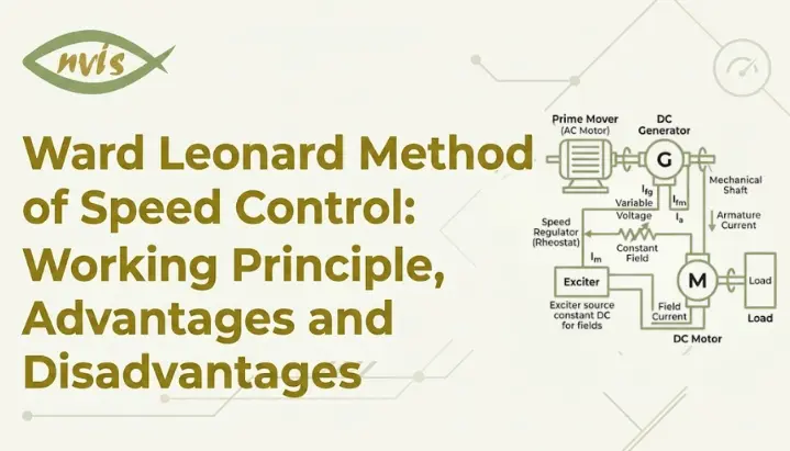
Ward Leonard Method of Speed Control: Working Principle, Advantages and Disadvantages

Posted on 20-08-202620-08-2026 by Tushar Saluja

TL;DR

This blog is for electrical engineering students, GATE and SSC JE aspirants, and freshers who want to understand Ward Leonard method of speed control with a clear, exam ready explanation rather than a dry textbook definition.
Ward Leonard system controls a DC motor’s speed by changing voltage fed to it, using a separate motor generator set instead of resistors or switches.
It became one of the smoothest and widest-range speed-control methods for DC motors and was widely used for decades in elevators, steel mills, mine hoists, cranes, and other demanding industrial applications.
A worked numerical example, comparison table, and India specific industrial context are included to help you connect theory to real plants and real exam questions.
Modern power-electronic drives, including thyristor DC drives and, where AC motors are used, VFDs, have largely replaced Ward Leonard systems.

Imagine trying to slow down a car by dragging your foot on the road instead of easing off the accelerator. It would work, technically, but you would waste a lot of energy as heat and wear out your shoe fast. Early speed control methods for DC motors had a similar problem. Engineers controlled speed by inserting resistors into the circuit, which wasted power as heat, gave a limited speed range, and could not push the motor above its normal speed smoothly.

Ward Leonard method of speed control solved this problem by changing strategy entirely. Instead of wasting energy through resistors, it changes voltage supplied to the motor directly, using a dedicated generator built just for that purpose. This single idea, controlling speed through variable voltage rather than variable resistance, became one of most important developments in the history of electric drives.

This blog breaks down Leonard’s system of speed control the way a mentor would explain it on a whiteboard: starting from everyday logic, moving into technical working, and ending with exact things you need for your GATE, SSC JE, or RRB JE preparation.

What Is the Ward Leonard Method of Speed Control?

Picture two water tanks connected by a pipe. If you want more water to flow through the pipe, you do not squeeze the pipe narrower and force water through it. You simply raise the water level in the first tank, and flow increases naturally with more pressure. Ward Leonard method applies exactly this logic to electricity.

In a DC motor, speed depends almost directly on voltage applied to its armature. Higher voltage means higher speed, and lower voltage means lower speed, as long as field current stays constant. So instead of restricting current with resistors, Ward Leonard method varies voltage itself, smoothly and continuously, using a generator whose output can be adjusted at will.

The Ward Leonard method of speed control was introduced by American engineer Harry Ward Leonard in 1891. His idea was simple but powerful. Take a constant speed AC or DC motor, couple it mechanically to a separately excited DC generator, and let that generator supply variable DC voltage to the motor you actually want to control. Change generator’s field current, and its output voltage changes. Change output voltage, and the controlled motor’s speed changes right along with it.

This is why the Ward Leonard control system is often called an armature voltage control method. The field of the controlled motor remains untouched. For speeds up to the base speed, the Ward Leonard system controls the motor through variable armature voltage while keeping the motor field approximately constant. For speeds above the base speed, motor field weakening can be combined with armature voltage control to achieve a wider speed range.

Three Machines Behind Ward Leonard System

To really understand how this system works, it helps to think of it as a small team of three machines, each with one job.

A driving motor is a constant speed machine that keeps everything running. It is usually a three phase induction motor or a synchronous motor, connected directly to the main AC supply, and it always spins at a fixed speed. Its only job is to provide mechanical power to turn the generator.

The generator is coupled mechanically to the driving motor, so it always spins at that same constant speed too. But its electrical output is not fixed. By adjusting the generator’s own field current through a small rheostat, its output voltage can be raised or lowered smoothly from zero to its rated value, and even reversed in polarity.

A controlled motor, sometimes labelled M1 in textbook diagrams, is an actual DC motor whose speed you want to control. It receives its armature supply directly from the generator, while its field winding is separately excited and kept constant. Since motor speed depends on armature voltage, and generator’s voltage is fully adjustable, the controlled motor’s speed becomes fully adjustable too.

The combination of the driving motor and generator is called the motor-generator (MG) set. Together with the controlled DC motor, it forms the basic Ward Leonard system.

How Speed Control Actually Happens

Here is where the system becomes genuinely elegant. A field regulator, a small rheostat connected to the generator’s field winding, is the only control operator needs to touch.

When the generator’s field current is zero, its output voltage is zero, and the controlled motor stays still. As the operator gradually increases field current using rheostat, the generator’s output voltage rises smoothly from zero. This voltage is applied directly to the controlled motor’s armature, so the motor starts rotating and speeds up in proportion to rising voltage.

Because the generator voltage can be increased gradually from zero, the motor can start smoothly while its armature current remains within the required limit. Therefore, a separate conventional starting resistor is not normally required in the Ward Leonard arrangement.

Reversing direction is just as elegant. By reversing the generator’s field current using a simple reversing switch, the polarity of the generator’s output voltage flips. This reverses current through the controlled motor’s armature, which reverses its direction of rotation, all while the motor generator set keeps spinning in the same direction throughout.

There is one more capability that made this system genuinely ahead of its time. During regenerative braking, the generator output voltage is reduced below the motor’s induced back EMF. The motor then operates as a generator and sends electrical power back through the Ward Leonard set. The generator operates in the opposite energy-conversion direction, ultimately allowing the prime mover to return energy to the AC supply. The Ward Leonard system has inherent regenerative braking capability, although the control arrangement must be designed to provide the required operating conditions.

Worked Numerical Example

Numbers make this concept concrete, and this is exactly the kind of question that shows up in GATE and SSC JE papers.

Suppose a separately excited DC generator in a Ward Leonard system is driven at a constant speed and generates 220 V when its field current is at rated value. This voltage is applied directly to armature of a separately excited DC motor whose armature resistance is 0.5 ohm and whose back EMF constant relates speed and flux such that at 220 V armature voltage and rated flux, motor runs at 1000 RPM while drawing a full load armature current of 20 A.

If the generator’s field current is reduced so that its output voltage drops to 110 V, and motor’s field flux is kept unchanged, new operating speed can be estimated using the relationship that speed is proportional to armature voltage minus armature resistance drop, divided by flux.

At 220 V: back EMF equals 220 minus (20 times 0.5), which is 220 minus 10, giving 210 V, corresponding to 1000 RPM.

At 110 V, assuming the motor continues to drive a constant-torque load, the armature current remains approximately 20 A for simplicity. Therefore, back
EMF = 110 − (20 × 0.5) = 100 V.

Since speed is proportional to back EMF when flux is constant, new speed works out to 1000 multiplied by (100 divided by 210), which is approximately 476 RPM.

This shows core exam skill directly: halving generator’s output voltage very nearly halves motor’s speed, since armature resistance drop is small compared to applied voltage. This proportional relationship between generator field current, generator voltage, and motor speed is exactly what most GATE and SSC JE numericals on Ward Leonard method are testing.

Ward Leonard Ilgner System

Large industrial loads rarely stay constant. A steel rolling mill or a mine hoist can demand a sudden, massive surge of power for a few seconds and then fall quiet again. Feeding these spikes directly from the AC supply would cause the whole plant’s voltage to sag and flicker, disturbing every other machine connected to the same supply.

Ward Leonard Ilgner system solves this by adding a flywheel and a slip ring induction motor to standard setup. During normal, light load periods, induction motor spins flywheel up to speed, storing rotational energy in it. The moment a sudden heavy load hits a controlled motor, that stored rotational energy gets released, so the flywheel momentarily slows down while it takes on part of the load itself, easing the burden on incoming supply. Once demand eases off again, the induction motor quietly spins the flywheel back up, ready for the next surge.

This arrangement reduces the peak power drawn from the AC supply by allowing the flywheel to supply part of the sudden overload. As a result, the required power rating of the supply-side equipment and driving motor can be reduced compared with a system designed to handle the entire peak load directly. This is precisely why the Ilgner variant found its home in heaviest industrial applications, including blooming mill drives and colliery winders, where individual drive units can run into megawatt range.

Advantages of Ward Leonard System

The reason this system dominated precision drives for nearly a century comes down to a genuinely strong list of benefits.

With appropriate armature-voltage control and motor field weakening, the Ward Leonard system can provide a wide speed range; traditional references commonly quote a maximum-to-minimum speed ratio of about 20:1 to 40:1, depending on the design and control arrangement.

Starting is gentle by nature, since the generator’s output voltage rises from zero, which means the controlled motor accelerates smoothly and no separate starter is required at all.

Speed regulation under load is excellent, meaning the motor holds its set speed closely even as mechanical load on it changes.

Regenerative braking is an inherent capability of the Ward Leonard system. When the motor is driven above the speed corresponding to the applied armature voltage, it can operate as a generator and return electrical energy through the drive system to the supply, provided the control arrangement supports regenerative operation.

Because of all this, the system was, and in some legacy installations still is, a natural choice for jobs demanding frequent starting, stopping, and direction reversal, such as elevators, rolling mills, and excavators.

Disadvantages of Ward Leonard System

None of these benefits came free, and drawbacks are exactly why modern plants have largely moved away from this method.

The system needs three full electrical machines instead of one, driving motor, generator, and controlled motor, which makes initial cost very high.

All that extra machinery also means a much larger physical footprint, heavier installation, a costlier foundation, and significantly more floor space than a compact modern drive would need.

Overall efficiency suffers because power is converted twice, first from AC to mechanical to DC in the generator, and then from DC to mechanical again in the controlled motor, and this inefficiency gets worse when the system runs under light load.

Three rotating machines mean more maintenance requirements, more noise during operation, and more potential points of mechanical or electrical failure.

These downsides are precisely why solid state alternatives eventually took over, a shift covered in detail in the next section.

Applications of Ward Leonard Method

Despite its bulk and cost, Ward Leonard system found a home wherever precision mattered more than efficiency or space.

Elevators relied on this system for decades, since it offered smooth speed control and consistent torque, until thyristor drives became widely available in the 1980s.

Steel rolling mills used it to drive rollers that shape red hot steel, where even slight speed inconsistency can ruin an entire batch of material.

Mine hoists and colliery winders depended on it for safely raising and lowering personnel and material through deep shafts, where smooth acceleration and reliable braking are safety critical.

Paper mills used it to keep multiple stages of the manufacturing process running at precisely synchronised speeds, since a mismatch anywhere along the line damages paper.

Beyond heavy industry, Ward Leonard-type motor-generator systems were also used in applications requiring precise electromechanical positioning, where extremely smooth, precise motion it offered was exactly what gun directing systems needed.

Ward Leonard System vs Modern DC and AC Drives

Comparing the classic Ward Leonard method against drives that eventually replaced it makes trade offs much clearer.

Parameter	Ward Leonard System	Modern VFD / Thyristor Drive
Number of machines needed	Three (driving motor, generator, controlled motor)	One (motor itself, plus a compact electronic converter)
Physical size and weight	Very large, heavy, needs significant floor space	Compact, panel mounted, minimal footprint
Initial cost	High, due to extra rotating machines	Lower, though power electronics add their own cost
Efficiency	Reduced by double energy conversion, worse at light load	High, since power electronic conversion has fewer losses
Maintenance	Frequent, due to brushes, bearings, and commutators on three machines	Minimal, mostly solid state with far fewer moving parts
Noise	Noticeable, from rotating machinery	Very low
Response speed	Smooth but mechanically limited	Extremely fast, controlled electronically
Typical modern use	Legacy installations, some heavy industrial retrofits	Standard choice in nearly all new industrial drives

Is the Ward Leonard Method Still Used in India Today?

Walk through a modern Indian steel plant today and you will rarely find a classic Ward Leonard motor generator set still running main rolling stands. Modern Indian steel plants increasingly rely on PLC-based automation and modern power-electronic drives, including DC drives and VFDs, for rolling-mill and other variable-speed applications, which deliver same precise, wide range speed control Ward Leonard system once provided, but from a fraction of footprint and with far less maintenance overhead.

This does not make the Ward Leonard method irrelevant. It remains genuinely important for three reasons. First, some older Indian mills, mine hoists, and elevator installations still run on legacy Ward Leonard equipment, and engineers maintaining these systems need to understand exactly how they work. Second, the Ward Leonard system is an important historical foundation for modern variable-speed drive technology, particularly electronic DC drives. Modern VFDs use a different approach based on power-electronic conversion and frequency control of AC motors. Third, and most practically for students, this topic is a recurring favourite in GATE, SSC JE, and RRB JE electrical engineering papers, which means skipping it is not really an option if you are preparing for these exams.

Understanding the Ward Leonard system, in other words, is less about maintaining old machines and more about understanding the DNA of every drive system that came after it.

Career Relevance of Ward Leonard Speed Control

Electrical drives and motor control are not just exam topics. They translate directly into real, well paying career paths in India, and understanding classical systems like Ward Leonard gives you a genuine head start when you move on to studying VFDs, servo drives, and industrial automation.

Career Relevance for Electrical Engineers

Understanding DC drives, motor control, regenerative braking, and industrial automation can help electrical engineering students build a foundation for careers in electrical drives, industrial automation, power electronics, and maintenance engineering.

Specialising further pays off significantly. Engineers who build expertise in industrial automation, PLCs, SCADA systems, or power electronics can access specialised career opportunities because these skills are widely used in modern industrial and electrical systems. Since the Ward Leonard method is an important milestone in the development of variable-speed electrical drives, a solid grasp of it makes concepts like VFD tuning, regenerative braking in EVs, and closed loop motor control noticeably easier to pick up later.

For students still deciding where to specialise, drives and automation remain one of more resilient tracks in Indian electrical engineering, since virtually every steel plant, cement plant, paper mill, elevator manufacturer, and EV company needs engineers who genuinely understand how motor speed control works, not just how to operate a VFD panel by trial and error.

GATE, SSC JE, and RRB JE Exam Relevance

Leonard method of speed control shows up consistently across Indian electrical engineering competitive exams, and it is worth knowing exactly what form these questions usually take.

Conceptual questions typically test whether you understand that this is fundamentally an armature voltage control method, applicable to DC shunt and separately excited motors, and that it is not used for series or universal motors. Expect direct statements to verify as true or false, along with questions asking you to identify which machine’s field current is actually being varied to control speed, since students often confuse generator’s field with motor’s field.

Numerical questions, similar to worked examples earlier in this blog, usually give you a generator voltage, an armature resistance, a load current, and a known speed at one voltage, then ask you to calculate the resulting speed at a different generator voltage. A key relationship to remember is that back EMF is proportional to speed when flux is constant, and back EMF equals applied voltage minus armature current times armature resistance.

Application based questions test whether you know why this method suits loads requiring frequent starting, stopping, and reversal, and why it offers inherent regenerative braking without any additional circuitry, a point that is very commonly tested precisely because it distinguishes Ward Leonard from simpler resistance based control methods.

Comparison questions often ask you to contrast Ward Leonard with other DC motor speed control methods, namely armature resistance control and field flux control, focusing on efficiency, cost, and speed range as key differentiators.

Conclusion

Ward Leonard method of speed control took a simple, honest idea, that motor speed follows armature voltage, and built an entire mechanical electrical system around delivering that voltage smoothly and reliably. It gave engineers a highly effective wide-range, bidirectional speed-control system for DC motors, decades before modern power electronics could perform similar functions in a much smaller package.

To summarise key points from this blog: system uses three machines working together, a driving motor, a generator, and a controlled motor, with speed adjusted purely through generator’s field current. It excels at smooth, wide-range, bidirectional control and inherent regenerative braking capability when operated in regenerative mode, but pays for this with high cost, large size, and lower efficiency compared to modern drives. Ilgner variant added a flywheel to handle heavy intermittent industrial loads without disturbing the main power supply. And while VFDs and thyristor drives have replaced it in nearly all new Indian installations, the underlying principle remains foundational to every modern variable speed drive in use today.

If you are preparing for GATE, SSC JE, or RRB JE, make sure you can explain the working principle in your own words, solve a voltage to speed numerically confidently, and list advantages and disadvantages without hesitation. That combination covers almost everything examiners ask about this topic.

FAQs

What is the Ward Leonard method of speed control used for?

Leonard method of speed control is used to smoothly control speed of a DC motor, in both directions of rotation, across a very wide range. It was historically used in elevators, steel rolling mills, mine hoists, cranes, and paper mills, wherever precise, sensitive speed control mattered more than cost or size.

Who invented the Ward Leonard control system?

The system was introduced by American electrical engineer Harry Ward Leonard in 1891, and it went on to become one of most influential drive control methods of the twentieth century.

Is the Ward Leonard method still used in India?

Rarely for new installations. Most Indian steel plants and industries have shifted to VFDs and thyristor based drives, which offer similar precise control from a much smaller footprint. However, some legacy elevators, mine hoists, and older mill drives still run on Ward Leonard systems, and underlying principle remains foundational to how modern drives work.

What is the difference between the Ward Leonard system and Ward Leonard Ilgner system?

The standard Leonard control system uses a motor generator set alone. Ilgner variant adds a flywheel and typically a slip ring induction motor, allowing the flywheel to absorb sudden heavy load demands and release stored energy back into the system, which smooths out supply current fluctuations in large industrial drives.

What are the main disadvantages of the Ward Leonard method of speed control?

The biggest drawbacks are high initial cost from needing three separate machines, large physical size and floor space requirements, reduced efficiency due to double energy conversion, and higher maintenance needs compared to modern solid state drives.

Does the Ward Leonard method work for DC series motors?

No. This is a common exam trap. Leonard system of speed control is designed for DC shunt motors and separately excited DC motors, where field can be held constant while armature voltage is varied. It is not a standard method used for series motors.

Why is the Ward Leonard method important for GATE and SSC JE preparation?

It is a recurring topic in DC machines and electrical drives sections of these exams, tested through conceptual questions, numericals relating voltage to speed, and comparison questions against other speed control methods. Understanding it thoroughly also builds foundation for later topics like VFDs and closed loop motor control.

Three Phase AC Voltage Controller Waveforms Explained: Modes, Working and Applications

Posted on 15-08-202615-08-2026 by Tushar Saluja

TL;DR

This blog is for electrical and electronics engineering students, freshers, and GATE, SSC JE, and RRB JE aspirants who want a clear, practical understanding of three phase AC voltage controller waveforms.
A three phase AC voltage controller uses six thyristors to control RMS voltage delivered to a three phase load without changing supply frequency.
output waveform depends on firing angle alpha, which falls into three distinct conduction modes, each producing a different chopped voltage shape.
A worked numerical example ties waveform theory to real RMS voltage and power calculations that students can reproduce in exams and labs.
The topic carries real weight in GATE Power Electronics and in India’s growing power electronics, EV, and industrial automation job market.

A three phase AC voltage controller is a circuit that controls the RMS value (effective value) of AC voltage supplied to a three phase load without changing the supply frequency. It uses six thyristors, two connected in anti parallel per phase, fired at a controlled delay angle after each natural commutation point. This blog explains how circuit operates, breaks down three conduction modes that shape its output waveforms, and connects theory to Indian industry applications, GATE exam relevance, and career paths in power electronics.

What Is a Three Phase AC Voltage Controller

Think about a fan regulator in your home. When you turn the knob, you are not changing the frequency of the AC supply coming into your house. You are simply controlling how much of each voltage cycle actually reaches the fan motor. Turn it down, and the fan gets a smaller “slice” of each cycle. Turn it up, and it gets more.

A three phase AC voltage controller does exactly this, but at an industrial scale, across three phases simultaneously, and using thyristors instead of a mechanical knob. Instead of a ceiling fan, load could be a large induction motor, an industrial heater bank, or a set of high power lamps drawing current from a three phase supply.

The main idea is simple. The controller does not convert AC into DC. It works only with AC and controls how much voltage reaches the load. It just “chops” each half cycle of input waveform, letting through only a controlled portion of it, so RMS voltage reaching load can be adjusted smoothly from close to full supply voltage down to nearly zero.

Because it controls AC voltage without changing it into DC, this circuit is also called an AC-to-AC converter or an AC voltage regulator. The primary keyword here, three phase AC voltage controller, refers to this exact family of circuits, and understanding its waveform behavior is the foundation for everything else in this topic.

How Circuit Works: Thyristors, Firing Angle and Natural Commutation Point

Before learning the waveforms, you should understand three basic ideas: a thyristor pair, the firing angle, and the natural commutation point.

Each phase of the controller uses two thyristors connected back to back, or antiparallel. One thyristor conducts during the positive half cycle of that phase’s voltage, and the other conducts during the negative half cycle. This antiparallel pairing is necessary because a single thyristor can only conduct current in one direction, but an AC load needs current flowing both ways across a full cycle.

A natural commutation point is the moment when one thyristor turns off and another takes over because the AC supply changes direction. It serves as the reference point from which the firing angle is measured. For a three phase system, this point repeats every 60 degrees because there are six such transitions in every 360 degree cycle, one for each thyristor.

The firing angle (α) is the delay between the natural commutation point and the moment the thyristor is switched on. If alpha is small, thyristor turns on almost as soon as it is able to, and load receives nearly full voltage. If alpha is large, thyristor turns on late in cycle, so it conducts for a shorter time, and load receives a smaller RMS voltage.

Two more terms matter here. A thyristor turns off automatically the moment its current falls to zero, which is called natural or line commutation. And for a thyristor to actually fire, two conditions must be true at the same time: its anode voltage must be higher than its cathode voltage, and a gate pulse must be present. Instead of sending one short gate pulse, engineers often send several pulses over a short period. This makes sure the thyristor turns on even if the exact switching time changes slightly and a single narrow pulse might be missed.

Three Phase AC Voltage Controller Waveforms: Mode I, II and III Explained

This is the most important part of the topic. Many textbooks become difficult here because they start with maths instead of explaining the idea first. Before math, picture what is physically happening: as you increase firing angle alpha, fewer thyristors are conducting at any given instant, and shape of chopped waveform changes character three distinct times. Power electronics engineers label these three characters Mode I, Mode II, and Mode III.

Mode I: 0° ≤ α < 60°

In this range, the controller behaves almost like an uncontrolled circuit. At any instant, either two or three thyristors are conducting simultaneously. Because nearly full waveform gets through, output closely resembles undelayed sine waves, only slightly clipped near the start of each half cycle. This mode delivers the highest RMS output voltage range, from full supply voltage down to roughly 96 to 97 percent of it as alpha approaches 60 degrees.

Mode II: 60° ≤ α < 90°

Here behavior changes noticeably. At any given moment, exactly two thyristors conduct, one from each of two different phases. There is no longer a window where three thyristors conduct together. The output waveform now has small gaps where the voltage becomes zero before the next thyristor turns on. This is the transition zone where the chopped nature of the waveform becomes visually obvious on an oscilloscope.

Mode III: 90° ≤ α < 150°

In this final mode, the thyristors do not conduct continuously. There are short periods when no current flows. Sometimes two thyristors conduct together, and sometimes none conduct at all, leaving load voltage at zero for stretches of cycle. output RMS voltage drops sharply through this range, falling from around 70 percent of supply voltage at alpha equals 90 degrees to nearly zero as alpha approaches 150 degrees, which is the theoretical extinction point for a purely resistive star connected load.

Worked Numerical Example

Suppose a three phase, star connected, three wire AC voltage controller supplies a balanced resistive load with R equal to 10 ohms, connected to a 380 volt line to line, 50 Hz supply, and firing angle alpha is set to 30 degrees.

Since α = 30° is in Mode I, almost the full supply voltage reaches the load. Phase voltage Vm here corresponds to a line to neutral RMS value of about 220 volts. At alpha equals 30 degrees, standard control characteristic tables for this configuration show output RMS phase voltage is close to 98.5 percent of supply phase voltage, giving an output of roughly 216 to 217 volts RMS per phase.

Using this output voltage, RMS load current per phase works out to approximately Vo,rms divided by R, and output power per phase follows from Vo,rms squared divided by R. For a balanced three phase load, total output power is simply three times per phase power. This is exactly the kind of calculation that appears in GATE and university exam papers, so working through it by hand, rather than only reading derivation, builds real exam readiness.

Now compare this to alpha equals 90 degrees on the same circuit. System shifts into Mode III, and output RMS voltage collapses to roughly 70 percent of supply value, which more than halves delivered power compared to alpha equals 30 degrees, since power scales with square of voltage.

Comparison Table: Single Phase vs Three Phase AC Voltage Controller

Parameter	Single Phase AC Voltage Controller	Three Phase AC Voltage Controller
Thyristors required	2 (one antiparallel pair)	6 (two per phase)
Firing angle range for full control	0° to 180°	0° to 150° for resistive star load
Number of conduction modes	Not applicable	Three distinct modes (I, II, III)
Typical applications	Lamp dimming, single phase heaters, small fan regulators	Three phase motor speed control, industrial heaters, soft starters
Harmonic content	Odd harmonics present	Odd harmonics present, triplen harmonics depend on connection type
Control complexity	Simple, single firing circuit	More complex, six coordinated firing circuits
Common connection types	Direct or with transformer	Star three wire, star four wire, or delta connected

Applications of Three Phase AC Voltage Controller in Industry

Three phase AC voltage controllers are used in industries where AC power needs to be controlled smoothly without converting it into DC. The most common application is limited speed control of induction motors, mainly in fan and pump applications where torque requirements permit voltage control used in fans, pumps, and conveyor systems, where the controller adjusts voltage fed to the stator to vary motor speed and torque within limits.

Industrial heating systems are another major use case, particularly in furnaces and ovens where precise temperature control depends on regulating RMS voltage delivered to heating elements rather than switching them fully on or off. Static VAR compensators and soft starters for large motors also rely on the same underlying phase control principle, using controlled firing of thyristors to limit inrush current during motor startup.

Lighting control for large scale industrial or commercial installations, where dimming needs to happen uniformly across all three phases, is a further application area, along with certain classes of certain thyristor-based AC voltage regulators used in industrial power control with sensitive equipment.

India Context: Industry, Employers and Regulatory Landscape

In India, three phase AC voltage controllers and a broader family of AC to AC power electronic converters are core building blocks in sectors that the government has been actively pushing: renewable energy integration, industrial automation, and electric mobility. Companies such as BHEL, L&T, Siemens, ABB, and Crompton Greaves design and manufacture equipment that relies on this class of thyristor based control, particularly for motor drives and industrial power quality equipment.

Government policies also play an important role. Bureau of Energy Efficiency and broader push toward energy efficient industrial motors under India’s national programs have increased demand for engineers who understand voltage and speed control at power electronics level, not just at mechanical or control systems level. As India’s manufacturing sector modernizes under initiatives like Make in India and Production Linked Incentive schemes for electronics and semiconductor manufacturing, practical skill of reading and designing around thyristor controlled AC waveforms remains directly employable.

Public sector undertakings such as NTPC, PowerGrid, and BHEL, along with private players expanding into EV charging infrastructure and grid scale power electronics, continue to hire electrical engineers with a solid grounding in power electronics fundamentals, of which three phase AC voltage controller is a standard part of undergraduate and GATE syllabus.

Career and Salary Guidance in Power Electronics (India, 2026)

The average salary for a Power Electronics Engineer in India currently stands close to eight lakh rupees per year, with a typical range roughly between five and a half lakhs and eleven and a half lakhs annually depending on experience and employer. At fresher level, entry into government and PSU roles through GATE typically corresponds to a fixed pay scale in the six to twelve lakh range, while private sector roles in EV and semiconductor adjacent power electronics work can pay significantly more once a few years of hands-on experience are added.

Engineers who learn power electronics, motor drives, and battery management systems usually have better career opportunities for EV and grid integration space are seeing some of the fastest salary growth in the Indian market right now, with experienced roles in this niche commanding substantially higher packages than generalist electrical engineering positions. Renewable energy, industrial automation with PLC and SCADA skills, and defence and aerospace power systems roles round out strongest career tracks for someone who has built a genuine understanding of AC voltage control and related power conversion topics.

For students planning their career path, practical advice is straightforward: a strong grip on power electronics fundamentals such as three phase AC voltage controller, combined with hands on simulation experience using tools like MATLAB or PSIM, and a competitive GATE score, opens doors to both well established PSU route and faster growing private sector opportunities in EV and renewable energy companies.

GATE / SSC JE / RRB JE Exam Relevance

Power Electronics is one of higher weightage sections in GATE Electrical Engineering paper, and AC voltage controllers fall squarely within its syllabus alongside rectifiers, choppers, and inverters. Questions on this topic typically test three things: ability to identify correct conduction mode for a given firing angle, ability to compute RMS output voltage or output power for a stated alpha, and conceptual understanding of thyristor firing and commutation.

For SSC JE and RRB JE aspirants, depth of numerical analysis expected is usually lower than GATE, but conceptual questions on thyristor operation, purpose of firing angle, and basic difference between single phase and three phase AC voltage controllers appear regularly in power electronics and basic electrical engineering sections of these exams.

For exams, first learn the three conduction modes and their firing angle ranges. Many questions can be answered by identifying the correct mode and their alpha ranges first, since a large share of objective questions can be answered correctly just by recognizing which mode a given firing angle falls into, without needing to solve full RMS voltage integral under exam time pressure.

Conclusion

A three phase AC voltage controller regulates AC power the same way a fan regulator does, just scaled up to industrial three phase loads using six coordinated thyristors instead of a single mechanical dial. The output waveform passes through three distinct conduction modes as firing angle alpha increases from 0 to 150 degrees, and recognizing these modes is key skill for both exam problems and real circuit analysis. This topic is important because it is asked in GATE exams and is also widely used in industry in India’s growing power electronics, EV, and industrial automation sectors, which makes it worth mastering properly rather than memorizing formulas. Work through worked examples in this blog on paper, try varying firing angles yourself, and you will find underlying logic becomes intuitive far faster than equations alone suggest.

FAQs

What is the difference between a three phase AC voltage controller and a rectifier?

A rectifier converts AC input into DC output, while a three phase AC voltage controller keeps output in AC form and only adjusts its RMS magnitude. Both use thyristors and firing angle control, but the controller never creates a DC link.

Why does a three phase AC voltage controller need six thyristors?

Each of three phases needs an antiparallel pair of thyristors to handle both positive and negative half cycles of that phase’s voltage, since a single thyristor conducts in only one direction. Three phases multiplied by two thyristors each gives six total.

What are three modes in three phase AC voltage controller waveforms?

Mode I covers firing angles from 0 to 60 degrees where two or three thyristors conduct together, Mode II covers 60 to 90 degrees where exactly two thyristors conduct at a time, and Mode III covers 90 to 150 degrees where conduction becomes intermittent and can drop to zero.

What is the maximum firing angle for a three phase full wave AC voltage controller with resistive load?

For a star connected three wire configuration with a balanced resistive load, practical extinction point is around 150 degrees, beyond which output voltage effectively falls to zero.

Is three phase AC voltage controller topic important for GATE Electrical Engineering?

Yes, it falls under Power Electronics section of GATE EE syllabus, which typically carries significant weightage, and questions frequently test conduction mode identification and RMS output voltage calculations.

Where are three phase AC voltage controllers used in Indian industry?

They are commonly used for three phase induction motor speed control, industrial heating and furnace applications, soft starters for large motors, and certain lighting and power quality applications in manufacturing plants across companies like BHEL, L&T, Siemens, and ABB.

What Is a Torsional Pendulum? Definition, Working Principle & Examples

Posted on 15-08-202615-08-2026 by Tushar Saluja

TL;DR

This is a blog for the beginners of engineering and physics, freshers and competitive exam aspirants (GATE, JEE, NEET, SSC JE, RRB JE) who want to understand the concept of a torsional pendulum at an easy level in a simple manner.
Many students find this topic confusing at first because the body rotates by twisting about its axis instead of swinging side to side like a simple pendulum.
Think of twisting a wire with your hand. The more you twist it, the more it resists. When you let go, it twists back, goes a little too far, and keeps moving back and forth for a while.
A torsional pendulum has a time constant of T = 2π√(I/κ) where I is the moment of inertia of the suspended object and κ (kappa) is the torsional constant of the wire.
This concept is used in mechanical watches, the Cavendish experiment, and some scientific instruments. It is also a common topic in GATE, JEE, and other engineering exams.

A torsional pendulum is a rigid body suspended by a thin wire or fibre. Instead of swinging, it rotates back and forth by twisting the wire. The wire’s elasticity creates a restoring torque that brings the body back to its original position. This topic is important in physics and engineering courses and is commonly asked in exams like GATE, JEE, and NEET.

This blog explains what a torsional pendulum is, how it works, its time period formula, how it differs from a simple pendulum, and where it is used in real life. You’ll also find a solved example and exam tips to help you understand the concept instead of just memorizing the formula.

What Is a Torsional Pendulum?

Think about twisting a wet towel after washing it. What happens when you hold one end and twist the other end of a towel? The towel pushes back because it wants to untwist. When you let go, it twists in the opposite direction. It keeps moving back and forth for a while before it finally stops.

The principle behind a torsional pendulum is the same as that of the towel, except that the “towel” is a thin wire, and the twisting effect applied to the pendulum is called torque.

A torsional pendulum is a rigid object, such as a disc or rod (a disc, rod or any symmetrical body) attached by means of a thin wire or fibre to a point at the top. Now, with the body slightly twisted around the wire’s axis, when it is released, the twisted wire produces a restoring torque that pulls the body back toward its original position. Because of its inertia, the body does not stop at its starting position. It moves a little past it, twists the wire in the opposite direction, and continues repeating the motion. This back and forth oscillatory movement is called torsional oscillation.

The key difference is that the object does not swing like a playground swing. Instead, it rotates around a fixed vertical axis but rather rotates around a fixed vertical axis, and this is what distinguishes the whole motion from the simple pendulum that most students are first introduced to in school physics.

Working Principle Behind a Torsional Pendulum

To understand what is happening physically, it helps to separate two ideas that are easy to mix up when you’re new to this: torque and torsion.

Torque is simply a twisting force. You can think of it as the turning version of a push or pull. Torsion means the resistance a wire or shaft creates when you try to twist it. When you twist wire in a torsional pendulum by a small angle θ (theta), wire develops an internal restoring torque that tries to bring it back to an untwisted state. This works much like Hooke’s law for springs, where stretching a spring generates a restoring force proportional to displacement.

For torsion, the restoring torque is:

τ = −κθ

In this case, the restoring torque is τ (tau) and angle of twist (in radians) is θ and the torsional constant of wire is κ which depends on the wire’s material, thickness, and length. A negative sign is just saying that torque is always in the opposite direction of the twist, which is why it is referred to as “restoring” torque.

After twisting and releasing the body, this torque restores the body toward its equilibrium position. Just as the swinging pendulum has momentum that propels it beyond its lowest position, the rotating object here has rotational inertia that propels it beyond the equilibrium angle, in the opposite direction. This is repeated, resulting in periodic, smooth oscillations: angular simple harmonic motion.

If we apply Newton’s second law for rotation, we get an equation that describes the motion. It follows the same pattern as simple harmonic motion but uses rotation instead of straight-line movement, it’s just written in angular terms.

Time Period of a Torsional Pendulum: Formula

Once the equation of motion is set up, comparing it with a standard simple harmonic motion equation gives a clean formula for the time period, time taken to complete one full oscillation.

T = 2π√(I/κ)

Where:

T is time period, measured in seconds
I is moment of inertia of suspended body about axis of rotation, measured in kg·m²
κ is torsional constant of wire, measured in N·m/rad

This formula tells you something important that’s easy to miss on first read: time period does not depend on the angle you twist your body through, as long as that angle stays small. Whether you twist the disc by 5 degrees or 15 degrees, it takes the same amount of time to complete one oscillation. This property is called isochronism, which means the time period stays the same for small twists. This is one reason mechanical watches can keep accurate time, since a wristwatch obviously can’t rely on gravity driven swinging while strapped to someone’s wrist.

Also worth noting: angular frequency ω (omega) of oscillation is given by ω = √(κ/I), and frequency f = 1/T. These three quantities, T, ω, and f, all describe same oscillation from different angles, and GATE and JEE numericals often ask you to convert between them.

Worked Numerical Example

Let’s apply formulas to a typical exam style problem, since seeing calculation once makes concepts far easier to recall later.

Problem: A disc has a moment of inertia of 0.05 kg·m² about its suspension axis. It is suspended from a wire with a torsional constant of 2 N·m/rad. Find the time period of the torsional pendulum.

Step 1: Write down known values. I = 0.05 kg·m² κ = 2 N·m/rad

Step 2: Substitute into formula. T = 2π√(I/κ) T = 2π√(0.05/2) T = 2π√(0.025) T = 2π × 0.158 T = 0.993 seconds (approximately 1 second)

Step 3: Interpret result. disc completes one full oscillation, twist one way, back through center, twist other way, and back to center, in roughly 1 second. If you doubled the moment of inertia (say, by attaching extra mass to the disc’s rim), the time period would increase by a factor of √2, since T is proportional to the square root of I.

Questions like this are common in GATE, JEE Main, and university exams, and the trick most students miss is forgetting to take the square root of the entire fraction I/κ before multiplying by 2π.

Torsional Pendulum vs Simple Pendulum: What’s Difference?

Students often confuse torsional and simple pendulums because both move back and forth and have similar time period formulas. But the reason they move is completely different and understanding this difference is very helpful in exam MCQs.

Feature	Simple Pendulum	Torsional Pendulum
Type of motion	Swings side to side (linear angular displacement)	Rotates back and forth about a fixed axis
Restoring force	Gravity (component of weight)	Torsion in wire (elastic restoring torque)
Formula for time period	T = 2π√(L/g)	T = 2π√(I/κ)
Depends on	Length of string (L) and gravity (g)	Moment of inertia (I) and torsional constant (κ)
Works in zero gravity	No, gravity is essential	Yes, since gravity plays no role in restoring torque
Real world example	Pendulum clock, playground swing	Mechanical watch balance wheel, Cavendish experiment

The most important difference to remember is this: a simple pendulum needs gravity to work, while a torsional pendulum does not depend on gravity at all. That’s exactly why torsional oscillators are used inside wristwatches, which move around constantly and can’t rely on a steady gravitational swing the way a wall clock can.

Real World Applications of Torsional Pendulums

This is the part where many students finally understand the concept because they see where it is used in real life.

Mechanical watches: balance wheel inside a mechanical watch is a small torsional pendulum, with a coiled hairspring providing restoring torque instead of a long wire. Because the oscillation period doesn’t depend on gravity or orientation, this is what lets a watch keep accurate time whether it’s lying flat on a table or strapped to a moving wrist.

Cavendish experiment: In 1798, Henry Cavendish used a torsion balance, essentially a torsional pendulum with two small masses on a suspended rod, to measure incredibly weak gravitational attraction between lead spheres. This experiment gave the first accurate measurement of universal gravitational constant G, and by extension, mass of Earth. extreme sensitivity of a torsional pendulum to tiny torques is what made this measurement possible at all.

Measuring modulus of rigidity: In physics and engineering labs, torsional pendulum experiment is a standard practical used to determine modulus of rigidity (shear modulus) of a wire’s material. By measuring the time period for known moments of inertia, students can work backward to calculate the wire’s torsional constant, and from that, material’s rigidity modulus. This exact experiment appears in most engineering physics lab manuals across Indian universities.

Finding moment of inertia of irregular bodies: Since I and κ are directly related through time period formula, a torsional pendulum setup can also be used other way around, to determine unknown moment of inertia of an irregularly shaped object by comparing its oscillation period to that of a known reference body.

Sensitive scientific instruments: Modern torsion balances are still used in precision measurements of tiny forces and in experimental physics. Gravitational wave detectors primarily use laser interferometry rather than torsion balances. Torsion balances are still used in modern physics experiments because a thin torsion fiber can detect extremely small twisting forces that many other sensors cannot measure.

Torsional Pendulum in GATE, JEE, NEET, and University Exams

In exams, questions about torsional pendulums usually come in a few common types generally fall into a few predictable categories, and knowing patterns in advance saves a lot of preparation time.

Conceptual MCQs often ask about the nature of the motion. A torsional pendulum undergoes angular simple harmonic motion because the restoring torque is directly proportional to the angular displacement.”Some MCQs test whether you know restoring torque comes from torsion, not gravity.

Direct numerical problems give you I and κ (or enough information to calculate them) and ask for time period, frequency, or angular frequency, exactly like the worked example above.

Derivation based questions, common in university semester exams and GATE Physics, ask you to derive expressions for a time period starting from the restoring torque equation, similar to how you’d derive T = 2π√(m/k) for a spring mass system.

Comparison questions test whether you can distinguish a torsional pendulum from a simple or physical pendulum, usually through a scenario based question rather than a direct definition.

For GATE Physics and Mechanical Engineering aspirants specifically, this topic connects closely with shafts and torsional stiffness in machine design, so understanding torsional pendulum well also helps when related topics show up later in strength of materials or vibrations papers.

Conclusion

A torsional pendulum is a rotational oscillator that is suspended from a wire that produces a restoring torque that is proportional to the angle of twist. Its time period, T = 2π√(I/κ), is independent of gravity, which is why it is used in mechanical watches, as well as in the Cavendish experiment to measure the gravitational constant of earth.

Try to understand the idea instead of memorizing the formula. The same concept appears in many other topics in physics and engineering. Now attempt to work on the numerical example above alone, then work through a few practice problems with varying values of I and κ, to start getting comfortable before the next exam.

FAQs

Q: What is a torsional pendulum in simple words?

A torsional pendulum is a rigid object, such as a disc or rod, suspended by a thin wire. The wire resists twisting and pulls the object back, making it rotate back and forth, causing repeated rotational oscillation.

What is the formula for the time period of a torsional pendulum?

The time period is given by T = 2π√(I/κ), where I is the moment of inertia of the suspended body and κ is the torsional constant of the wire.

What is the difference between a torsional pendulum and a simple pendulum?

A simple pendulum swings due to gravity, while a torsional pendulum rotates due to elastic restoring torque of a twisted wire. A torsional pendulum doesn’t need gravity to function, which is why it’s used in wristwatches.

Is motion of a torsional pendulum simple harmonic motion?

Yes, it is angular simple harmonic motion, since restoring torque is directly proportional to angular displacement, following the same mathematical pattern as linear SHM, just applied to rotation instead of straight line movement.

Where is a torsional pendulum used in real life?

Torsional pendulums are used in mechanical watch balance wheels, historic Cavendish experiment for measuring gravitational constant, physics lab experiments to determine a wire’s modulus of rigidity, and modern precision torsion balances used in scientific research.

Why does the time period of a torsional pendulum not depend on the twist angle?

As long as angular displacement stays small, restoring torque remains proportional to angle (following Hooke’s law for torsion), which keeps motion in true simple harmonic form. This property, called isochronism, means oscillation always takes the same time regardless of how far the body was twisted initially.

Unsymmetrical Fault in Power System: Types, Analysis & Protection

Posted on 01-08-202603-08-2026 by Tushar Saluja

TL;DR

This blog is for engineering students, freshers, and anyone learning power systems for the first time who wants to understand what an unsymmetrical fault is, why it matters, and how engineers analyze and protect against it.
An unsymmetrical fault is any short circuit that does not affect all three phases of a power system equally, unlike a symmetrical fault, which hits all three phases the same way.
three standard types are single line to ground, line to line, and double line to ground faults, and each one is analyzed using a technique called symmetrical components.
Symmetrical components break a messy, unbalanced fault into three clean, balanced pieces called positive, negative, and zero sequence networks, which makes math manageable.
In India, this topic has real 2026 relevance because the country’s renewable energy expansion and grid modernization efforts, along with regulations from the Central Electricity Authority (CEA), depend on how well solar and wind plants ride through unsymmetrical faults.

An unsymmetrical fault in a power system is a short circuit condition where three phases of a three phase electrical network no longer carry equal and balanced currents. It is the most common type of electrical fault encountered in transmission and distribution systems, accounting for the vast majority of short-circuit faults studied by protection engineers. Unlike a symmetrical fault, where all three phases are affected identically and the system remains balanced even during disturbance, an unsymmetrical fault introduces an imbalance that complicates both physics of the system and mathematics used to analyze it.This guide explains what an unsymmetrical fault is, why it behaves differently from a balanced fault, and how engineers use a technique called symmetrical components to make sense of it. It covers three standard fault types, walks through a worked numerical example, and connects topics to what is actually happening in India’s power grid in 2026, including renewable energy integration, CEA regulations, and career paths available to students who want to specialize in this area.

What Is an Unsymmetrical Fault, Really?

Picture three friends walking side by side at the exact same pace, perfectly in step with each other. That is roughly what a healthy three phase power system looks like. Three phases, usually labeled A, B, and C, carry currents that are equal in size and evenly spaced apart in timing, 120 degrees apart to be precise. This balance is what makes three phase power so efficient and predictable.Now imagine one of those three friends trips and falls. The other two keep walking, but the group is no longer in step. Something similar happens during an unsymmetrical fault. One or two phases get disrupted, usually because a conductor touches ground, or two conductors accidentally touch each other, while the remaining phases continue operating closer to normal. The result is a system that is suddenly unbalanced.This is the core definition worth remembering: an unsymmetrical fault, sometimes called an unbalanced fault or asymmetrical fault, does not treat all three phases equally. That single fact is what separates it from a symmetrical fault and is also why it needs a completely different analytical approach, which we will get into shortly.Unsymmetrical faults are not rare edge cases. Industry data consistently shows that approximately 70% of faults in power systems are single line to ground faults alone, and when you add line to line and double line to ground faults into the mix, unsymmetrical faults make up the vast majority of everything that protection engineers deal with. Symmetrical faults, where all three phases fail together, are actually rare, severe exceptions rather than everyday reality.

Symmetrical vs Unsymmetrical Fault: Spotting Difference

Before going deeper into unsymmetrical faults, it helps to draw a clear line between two broad fault categories, because students often mix them up early on.A symmetrical fault, sometimes called a balanced fault or a three phase fault, involves all three phases simultaneously and equally. Think of it as all three friends tripping at once, in perfect sync. system stays balanced throughout the entire fault event, even though it is now short circuited. This actually makes math simpler in one specific way: for a symmetrical three phase fault, only the positive sequence network is involved in analysis, because there is no imbalance to account for.An unsymmetrical fault, on other hand, involves only one or two of three phases. The system becomes unbalanced the moment fault occurs, and that imbalance has to be captured mathematically using additional tools beyond what a simple balanced analysis can offer.Here is a simple comparison to keep two straight:

Aspect	Symmetrical Fault	Unsymmetrical Fault
Phases affected	All three equally	One or two only
Frequency of occurrence	Rare, most severe	Very common (majority of faults)
System balance during fault	Remains balanced	Becomes unbalanced
Analysis method	Positive sequence network only	Positive, negative, and zero sequence networks
Typical example	Three phase short circuit	Single line to ground fault

Keep this table in mind, because everything discussed from this point forward assumes you understand that an unsymmetrical fault disrupts balance that three phase systems depend on, and that disruption is precisely what makes analysis interesting.

Types of Unsymmetrical Faults You Need to Know

Engineers generally group unsymmetrical faults into three standard categories, and it helps to think of them in increasing order of complexity rather than trying to memorize them as a random list.

Single Line to Ground (LG) Fault

This is the most frequent fault type you will encounter in any power system, and understanding it first makes everything else easier to follow. A single line to ground fault happens when one phase conductor comes into contact with ground, or with a grounded structure like a transmission tower.In the real world, this often happens because a vehicular accident causes one of the phase conductors to fall and come in contact with earth, or it may be caused by tree branches, or it could be caused by flashovers across dusty insulators during rain showers. If you have ever seen a fallen power line during a storm, there is a good chance you were looking at exactly this kind of fault.Because only one phase is disturbed, the other two phases largely retain their normal voltage and current behavior, but the overall system still becomes unbalanced enough to require careful analysis.

Line to Line (LL) Fault

A line to line fault occurs when two phase conductors touch each other directly, without involving ground at all. This might happen due to conductor clashing during high winds, insulation failure between two phases, or physical damage that brings two live conductors into contact.Since two phases are shorted together while the third remains isolated from fault, current and voltage relationships look quite different from a single line to ground fault, even though both are classified as unsymmetrical.

Double Line to Ground (LLG) Fault

This is where two phase conductors touch each other and simultaneously make contact with ground. It is less common than previous two types but tends to produce more severe fault currents because there are now multiple paths for current to flow, both between two faulted phases and from those phases down to ground.Of standard unsymmetrical fault types, double line to ground fault is generally considered most severe, sitting just below fully symmetrical three phase fault in terms of overall impact on the system.

Why LLLG Is Not Same as LLL

Here is a distinction that trips up almost every student the first time they encounter it, so it deserves its own dedicated section rather than being buried inside a definition.A three phase fault, written as LLL, involves all three phases shorting together but does not necessarily involve ground. This is a symmetrical fault. A three phase to ground fault, written as LLLG, involves all three phases shorting together and simultaneously connecting to ground. Some references distinguish between LLL and LLLG faults. In practice, both are symmetrical faults, and whether LLLG produces a higher fault current depends on the system grounding and sequence impedances rather than being universally more severe.The confusing part is that both LLL and LLLG are technically symmetrical, because all three phases are still treated equally in both cases. Whether or not ground is involved does not break symmetry, since ground connection affects all three phases the same way. This is different from LLG, double line to ground fault discussed earlier, where only two of three phases are involved, which is what makes LLG genuinely unsymmetrical.If you keep one rule in your head, make it this one: symmetry depends on whether all three phases are treated identically, not on whether ground is involved. That single distinction resolves most of the confusion between these fault categories.

Real Reason Unsymmetrical Faults Need Special Math

At this point you might be wondering why engineers cannot just analyze an unsymmetrical fault the same way they analyze a symmetrical one. The honest answer is that they tried, historically, and it turned into an enormous mess.When a system is perfectly balanced, whether under normal operation or during a symmetrical fault, you can analyze just one phase and assume the other two behave identically, just shifted in time. This is called per phase analysis, and it is the reason three phase power calculations are usually so manageable.The moment a fault becomes unsymmetrical, that shortcut disappears. Each phase now has a different current and voltage, which means you are stuck solving three separate, interconnected equations simultaneously for every single fault scenario. Every different fault type would need its own completely different set of equations, and complexity grows fast. A tool built to compare this exact problem notes that without symmetrical components, each fault type would require solving a different set of simultaneous equations in phase domain, vastly increasing computational complexity and opportunity for error.This is exactly the problem that symmetrical components were invented to solve, and it is why technique has remained the backbone of fault analysis for more than a century.

Symmetrical Components: Trick That Makes This Manageable

The method of symmetrical components was developed by an engineer named Charles Leggett Fortescue back in 1918, and it remains, even in 2026, standard technique taught in every power systems course and used in every commercial fault analysis software package.Here is the core idea in plain language. Instead of trying to directly solve three unequal, unbalanced phase currents at once, Fortescue proved that any unbalanced set of three phasors can be broken down into three separate balanced sets, each of which is much easier to analyze individually. Once you solve each balanced set on its own, you simply add them back together to get a real, unbalanced answer.These three balanced sets are:Positive sequence: Three phasors of equal magnitude, spaced 120 degrees apart, rotating in normal a b c sequence. This represents the system behaving exactly like it should under normal balanced conditions, and it is the only sequence present during normal healthy operation.Negative sequence: Three phasors of equal magnitude, also spaced 120 degrees apart, but rotating in reverse a c b sequence. Negative sequence currents only appear when there is an imbalance in the system, which is exactly why protection engineers use them as such a reliable indicator that something has gone wrong.Zero sequence: Three phasors that are equal in magnitude but have no phase displacement between them at all, meaning they all point in the same direction at the same time. Zero sequence current only flows when there is a path to ground, which is why it shows up specifically during ground faults.Think of it like separating a smoothie back into its original ingredients. Once blended, the mixture looks impossible to untangle. But mathematically, symmetrical components let engineers “unblend” unbalanced fault into three clean, separate ingredients, positive, negative, and zero sequence, work with each one individually using simple balanced system math, and then blend results back together at end to get true fault current and voltage at every phase.

Why This Actually Works: Sequence Networks

Each sequence component gets its own equivalent circuit, called a sequence network, built from impedances of generators, transformers, and transmission lines in the system. During normal operation, only the positive sequence network carries current, since the system is balanced and there is nothing to trigger negative or zero sequence components.The moment an unsymmetrical fault occurs, three sequence networks get connected to each other at fault location, and exactly how they are connected depends entirely on which type of fault has occurred. This connection pattern is genuinely elegant once you see it laid out. As one educational resource puts it, connecting sequence networks correctly for each fault type is a sort of calculation that has to be done whenever a line is installed or modified, so that protective relaying can be set properly.Here is how three standard unsymmetrical faults translate into sequence network connections:For a single line to ground fault: All three sequence networks, positive, negative, and zero, are connected in series with each other.For a line to line fault: Only positive and negative sequence networks are involved, connected in parallel opposition to each other. Zero sequence plays no role here, because there is no path to ground.For a double line to ground fault: The positive, negative, and zero sequence networks are interconnected according to the double line-to-ground fault conditions. Many textbooks represent this as the positive sequence network connected in series with the parallel combination of the negative and zero sequence networks, but the exact representation depends on the derivation and equivalent circuit used. This is the most complex connection of three, which lines up with the double line to ground being the most severe of standard unsymmetrical fault types.Once you have correct sequence network connection for a given fault type, calculating fault current becomes a matter of straightforward circuit analysis on that connected network, nothing more exotic than Ohm’s law applied to an equivalent circuit.

A Worked Example: Single Line to Ground Fault

Theory only really clicks once you have worked through an actual number, so here is a simplified single line to ground fault calculation using the kind of values you would see in a textbook problem or an early lab exercise.Consider a generator with following per unit sequence impedances, all referred to a common base:

Positive sequence impedance, Z1 = 0.15 per unit
Negative sequence impedance, Z2 = 0.15 per unit
Zero sequence impedance, Z0 = 0.05 per unit
Pre fault voltage, V = 1.0 per unit

Since a single line to ground fault connects all three sequence networks in series, total fault current in sequence domain is calculated by dividing pre fault voltage by sum of all three sequence impedances:I1 = I2 = I0 = V / (Z1 + Z2 + Z0)I1 = I2 = I0 = 1.0 / (0.15 + 0.15 + 0.05) = 1.0 / 0.35 = 2.857 per unitSince actual fault current at faulted phase is three times zero sequence current for this specific fault type, total fault current works out to:If = 3 × I0 = 3 × 2.857 = 8.571 per unitThis example intentionally uses round, simplified numbers to make the underlying pattern visible. Real fault studies performed by protection engineers use exact system data pulled from generator nameplates, transformer test reports, and transmission line parameters, then run through specialized short circuit analysis software rather than hand calculation. But underlying logic, adding up sequence impedances and dividing into pre fault voltage, remains exactly the same whether you are solving it by hand in a classroom or running it through a computer model for a real substation.

Effects of Unsymmetrical Faults on Power System

Understanding what actually happens to a power system during an unsymmetrical fault helps explain why protection engineers take this topic so seriously.Voltage sag and swell: phases involved in fault typically experience a voltage sag, a temporary drop below normal voltage, while unaffected phases can sometimes see a voltage swell, a temporary rise above normal. Sensitive equipment connected anywhere near fault location can be damaged or tripped offline by these swings if protection does not respond quickly enough.Current imbalance and overheating: Because current is no longer evenly distributed across three phases, some conductors and windings end up carrying more current than they were designed for. Sustained current imbalance generates excess heat, which gradually degrades insulation and shortens working life of transformers, motors, and generators connected to the system.Negative sequence heating in rotating machines: This deserves special mention because it specifically affects generators and large motors. Negative sequence current, remember, only exists during unbalanced conditions, creating a magnetic field that rotates in opposite direction to the machine’s normal rotation. This induces double frequency currents in the rotor, which generate intense localized heating that standard thermal protection is not always designed to catch quickly enough. This is exactly why negative sequence relays exist as a dedicated protection element in most modern generator protection schemes.System stability risks: In severe or prolonged cases, an unsymmetrical fault can push generators out of synchronism with the rest of the grid, potentially triggering cascading failures across a wider area if protection systems do not isolate fault fast enough.

How Engineers Protect Against Unsymmetrical Faults

Detecting an unsymmetrical fault quickly and isolating it before it causes wider damage is the entire purpose of a protection system, and this is where symmetrical components move from being a purely academic exercise into something engineers rely on every single day.Negative sequence relays specifically monitor for presence of negative sequence current, which, as covered earlier, only appears during unbalanced conditions. Since negative sequence current is essentially zero during healthy balanced operation, even a small amount is a highly reliable signal that something has gone wrong, which is exactly why protective relays utilize symmetric components for fault detection, and specifically why during normal operation, zero sequence current is very small, so a high current value is a convenient and reliable indicator of a ground fault.Distance protection measures impedance between relay location and fault point, and modern distance relays use sequence quantities to correctly classify which type of unsymmetrical fault has occurred, which in turn determines how quickly and in what manner circuit breaker should trip.Differential protection compares current entering and leaving a protected zone, such as a transformer or a section of transmission line, and trips instantly if two do not match within an unbalanced fault scenario, since any mismatch signals that current is escaping through an unintended path.Overcurrent protection with ground fault elements specifically watches for zero sequence current, which as discussed only flows when there is a path to ground, making it particularly effective at catching single line to ground faults quickly.Modern digital relays typically calculate all three sequence components in real time from raw phase currents and voltages they measure, then apply logic based on which sequence components are elevated to determine both fault type and its approximate location. This is the same symmetrical components theory from 1918, still doing exactly the job it was designed for, just running on a microprocessor instead of being worked out with pencil and paper.

Why This Matters Right Now in India’s Power Grid

Unsymmetrical fault analysis is not just an exam topic. In 2026, it sits at the center of one of the biggest engineering challenges facing India’s power sector, and understanding why will make the rest of this topic feel a lot less abstract.India has committed to genuinely ambitious renewable energy targets, with Government of India’s vision supporting integration of 450 GW Renewable Energy into National Grid by 2030 and an ambitious target of 2100 GW of Renewable energy by 2047. Solar and wind plants, unlike traditional coal or hydro generators, behave very differently during faults, and unsymmetrical faults specifically create real headaches for inverter based control systems these renewable plants depend on.This is exactly why the Central Electricity Authority, India’s apex technical regulator for the power sector, has built explicit requirements around this exact problem into national grid codes. Generating stations connecting to Indian grid must demonstrate ride through capability for balance and unbalanced faults (LVRT and HVRT), meaning a solar or wind plant has to remain connected to grid and continue operating even while an unsymmetrical fault is occurring nearby, rather than simply tripping offline moment voltage dips or spikes.CEA has also moved to formalize protection coordination across the entire national grid. Under current grid code, a uniform protection protocol is required for users of grid for proper coordination of protection systems in order to protect equipment from abnormal operating conditions, isolate faulty equipment, and avoid unintended operation of protection systems, and this Uniform Protection Protocol applies to all Regional entities, State, Central, and Private Generating Companies, Generating Stations, SLDCs, RLDCs, CTU, STUs, Transmission Licensees, and RPCs connected at 220 kV and above.More recently, CEA has extended this safety first approach into fast growing Battery Energy Storage System space as well. New 2026 regulations require BESS installations to follow a two fault tolerance design, ensuring systems remain safe even in event of two independent failures, along with protection against overcharging, deep discharge, short circuits, and operation beyond prescribed temperature limits, taking effect from April 2027.Put simply, every solar farm, every wind installation, and every battery storage project being commissioned across India right now has to prove, on paper and in testing, that it can survive an unsymmetrical fault without destabilizing the grid. This is the exact topic covered in this guide, now playing out at national scale.

Career Paths: What This Topic Means for Your Future

If you have made it this far, there is a good chance the underlying question in your mind is practical: does understanding unsymmetrical faults actually lead anywhere in terms of a career? The honest answer is yes, and demand is only growing as India’s grid gets more complex.Protection and relay engineering is the most direct career path connected to this exact topic. Protection engineers are people who calculate fault currents, set relay coordination parameters, and design protection schemes that keep the grid stable. Entry level protective relay engineer roles in India typically start in range of ₹3 to ₹6 LPA, with senior power systems engineers commanding significantly more, averaging around ₹18.4 LPA nationally and reaching approximately ₹20.5 LPA in cities like Bangalore where demand from grid modernization projects is particularly strong.POWERGRID Corporation of India Limited, a Maharatna public sector enterprise and one of largest transmission utilities in world, remains single largest direct employer for students entering this field through annual GATE based recruitment process, hiring Engineer Trainees and Assistant Engineer Trainees in Electrical and Electronics disciplines with starting pay around ₹50,000 to ₹60,000 per month during training, moving into E2 and E3 executive scales afterward. Beyond POWERGRID, state transmission utilities including HVPNL, RVPNL, and MAHATRANSCO regularly recruit engineers into similar protection focused roles.Global equipment manufacturers with a significant Indian presence, including Siemens, ABB, and Schneider Electric, hire electrical engineering graduates for relay design, testing, and system protection studies, often providing structured training programs that directly build on symmetrical components theory covered in this guide.Relevant skills and tools worth building as a student include familiarity with short circuit analysis software such as ETAP, PSS/E, and DIgSILENT PowerFactory, since these are industry standard platforms used to run exact fault calculations discussed in this guide at real substation scale. A solid grasp of per unit systems, single line diagrams, and relay coordination principles will also serve you well in interviews for these roles.Whether you pursue a core electrical engineering role at a utility, a specialized protection engineering position with an equipment manufacturer, or move into the renewable energy sector where fault ride through compliance is now a mandatory requirement, fundamentals covered in this guide form the technical bedrock entire career path is built on.

Emerging Trends: Where This Topic Is Headed

A few developments are actively reshaping how unsymmetrical fault analysis and protection get handled going forward, and being aware of them will serve students well beyond graduation.Grid forming inverters are increasingly being deployed for renewable plants specifically because they handle unsymmetrical faults more gracefully than older grid following inverter designs, actively injecting reactive power to support the grid during a fault rather than simply riding it out passively.Wide area monitoring using synchrophasors is giving grid operators real time visibility into sequence components across the entire network rather than just at a single substation, enabling faster and more coordinated responses to unsymmetrical fault events across large geographic areas.AI assisted fault classification is beginning to supplement traditional sequence component based relay logic, using pattern recognition trained on historical fault data to classify fault type and location even faster than conventional algorithms, though underlying symmetrical components theory remains the foundation these newer systems are built on top of.Extended data retention requirements are also becoming standard practice for renewable installations, with newer CEA technical standards requiring plants to store operational and fault data for extended periods with high resolution recording, specifically to support detailed post fault analysis and continuous improvement of protection settings over time.None of these trends replace fundamentals covered in this guide. If anything, they make a solid understanding of symmetrical components and sequence networks more valuable, not less, because every one of these newer technologies still has to speak the same underlying mathematical language when it comes to describing an unsymmetrical fault.

Conclusion

An unsymmetrical fault is ultimately about one simple idea with genuinely far reaching consequences: a three phase power system that suddenly stops treating its three phases equally. Whether that imbalance comes from a single line to ground fault, a line to line fault, or a double line to ground fault, underlying physics creates a mess that direct per phase analysis simply cannot untangle on its own. Symmetrical components solve this by breaking unbalanced mess into positive, negative, and zero sequence networks, each individually balanced and manageable, then recombining results to reveal true fault behavior across every phase.This is not purely theoretical knowledge confined to a textbook chapter. It is exact mathematics running inside every protective relay guarding India’s transmission and distribution network today, and it is the same framework Central Electricity Authority now requires every new solar, wind, and battery storage installation to satisfy before being allowed to connect to the national grid. For a student building a foundation in power systems, mastering unsymmetrical fault analysis is not just about passing an exam. It is about understanding the exact mechanism that keeps lights on across an entire country, and it opens a genuinely strong career path in protection engineering, grid operations, and the renewable energy sector that is actively hiring for these exact skills right now.

FAQs

Q: What is an unsymmetrical fault in a power system?

An unsymmetrical fault is a type of short circuit where three phases of a power system are affected unequally, unlike a symmetrical fault which involves all three phases identically. three standard types of unsymmetrical faults in a power system are single line to ground, line to line, and double line to ground faults.

Q: What is the difference between a symmetrical and an unsymmetrical fault?

A symmetrical fault involves all three phases equally and keeps the system balanced even during fault, while an unsymmetrical fault involves only one or two phases and creates an imbalance. Symmetrical faults are rarer but generally more severe, while unsymmetrical faults are far more common, with single line to ground faults alone accounting for roughly 70 percent of all faults in a typical power system.

Q: Why are symmetrical components used for unsymmetrical fault analysis?

Symmetrical components break an unbalanced, unsymmetrical fault into three separate balanced sequence networks, positive, negative, and zero sequence, which can each be analyzed using simple balanced system techniques and then recombined to find true fault current and voltage. Without this method, engineers would need an entirely different, far more complex set of equations for every single fault type.

Q: Which unsymmetrical fault is most common in power systems?

Single line to ground fault is by far the most common type of unsymmetrical fault, typically caused by fallen conductors, tree contact, or insulator flashovers, and it accounts for the large majority of faults encountered on real transmission and distribution networks.

Q: How does unsymmetrical fault analysis apply to renewable energy projects in India?

Indian grid codes now require solar, wind, and battery storage plants to demonstrate fault ride through capability for unbalanced faults before connecting to the national grid, directly under CEA regulations. This means the plant must stay connected and continue supporting the grid during an unsymmetrical fault rather than disconnecting immediately, making this exact topic a mandatory compliance requirement for any renewable project commissioned in India today.

Q: What career opportunities exist for students who understand unsymmetrical fault analysis?

Students with a strong grasp of unsymmetrical fault analysis can pursue protection and relay engineering roles at utilities like POWERGRID, equipment manufacturers such as Siemens and ABB, or renewable energy companies that need to demonstrate grid code compliance. Entry level protective relay roles in India typically start around ₹3 to 6 LPA, with power systems engineers earning considerably more as they gain experience with tools like ETAP and PSS/E.

Tags: Unsymmetrical Fault in Power System, Unsymmetrical Faults

Sumpner’s Test of Transformer: Working Principle, Circuit, and Procedure Explained

Posted on 01-08-202601-08-2026 by Tushar Saluja

TL;DR

This blog is for engineering students, freshers, and anyone preparing for GATE, SSC JE, RRB JE, or discom JE exams who wants to actually understand Sumpner’s test, not just memorize it.
Sumpner’s test (also called back to back test) lets you find a transformer’s iron loss and copper loss together, at full load, without connecting any real load to it.
It works by connecting two identical transformers so their secondaries cancel each other’s voltage, which tricks the system into simulating full load current while actual power drawn from supply stays tiny.
Two wattmeters do real work here one reads combined iron loss, other reads combined copper loss at full load, and a simple worked example later in this blog shows exactly how those numbers turn into efficiency and voltage regulation.
With India adding record transformer capacity through grid expansion projects in 2026, understanding this test isn’t just exam prep, it’s a real skill that shows up in testing labs at BHEL, POWERGRID, Siemens India, and CG Power.

Picture two friends trying to test how much weight a bridge can hold. Building a full scale replica bridge and loading trucks onto it would work, but it would cost a fortune and waste a huge amount of material just for one test. Now imagine there was a clever way to simulate the exact same stress on a bridge, using almost no material at all. That is essentially what Sumpner’s test does for transformers.

Sumpner’s test, also known as back to back test, is a method used to determine efficiency, voltage regulation, and heating behavior of a transformer under full load conditions, without ever connecting a real load to it. It solves a problem that has bothered electrical engineers for over a century: how do you test something as large as a power transformer at full load, when arranging that load in real life is expensive, wasteful, and sometimes just not possible.

This blog breaks concepts down from scratch. You will learn why this test exists, how circuit is set up, why physics behind it actually works, how to calculate efficiency and regulation from real readings, and why this topic still matters heavily in 2026, both for competitive exams and for real jobs in India’s fast growing power sector.

Why Do We Even Need a Test Like This?

Before understanding Sumpner’s test, it helps to understand the problem it was built to solve.

Every transformer loses some energy while it works. This loss shows up as heat, and it comes from two sources. First is iron loss (also called core loss), which happens inside a transformer’s core simply because it is carrying a changing magnetic field, whether or not any load is connected. Second is copper loss, which happens in windings because current flowing through wire generates heat, and this loss grows as load increases.

To measure these losses individually, engineers normally use two simpler tests: open circuit (OC) test and short circuit (SC) test. OC test gives you iron loss, and SC test gives you copper loss. Between two, you get a complete picture of the transformer’s equivalent circuit.

Here is the catch. In real operation, a transformer does not experience iron loss and copper loss separately. It experiences both at same time, continuously, while carrying its actual load. So while OC and SC tests are great for calculating losses on paper, they cannot tell you how hot a transformer will actually get when it is running under genuine full load for hours. That missing piece is temperature rise, and it matters enormously for large transformers, because overheating is one of fastest ways to damage insulation and shorten a transformer’s life.

So the real question becomes this: how do you load a transformer to its full rated capacity, long enough to observe realistic heating, without burning through massive amounts of electricity on an artificial load? This is exactly the gap that Sumpner’s test fills.

Core Idea: Making Two Transformers Load Each Other

Here is where analogy becomes useful again. Instead of using one giant external load to stress test a transformer, what if you could make two identical transformers push against each other, so that one effectively becomes a load for the other?

That is precisely the trick behind Sumpner’s test. It is sometimes even called regenerative test, because most of the power circulating between two transformers gets returned to the system rather than wasted, similar to how two people arm wrestling exert real force on each other without needing a third person to push against them from outside.

For this test to work, you need two transformers that are identical in rating, turns ratio, and impedance. This is a genuine limitation, since not every lab or testing facility has two matching transformers available, especially for large custom built power transformers. But wherever this condition can be met, the payoff is huge: you get a full load test using only a small fraction of actual full load power.

How Circuit Is Actually Connected

Now let’s get into wiring itself, one step at a time, because this is where most explanations jump too fast.

Take two identical transformers, call them T1 and T2. Their primary windings are connected in parallel and connected directly to normal rated supply voltage and frequency, exactly as they would be in real operation. So far, this is nothing unusual.

An interesting part happens on the secondary side. secondary windings of T1 and T2 are connected in series, but with their polarities deliberately opposed to each other. In plain terms, voltage induced in one secondary winding is arranged to cancel out voltage induced in another.

Since both transformers are identical, their induced secondary voltages are equal in magnitude. When you connect them in opposition, those two equal and opposite voltages cancel each other out almost perfectly. net voltage around that secondary loop becomes zero.

Before starting the test, this connection has to be verified. Engineers do this by taking two secondary terminals and joining them together, then measuring voltage across the remaining two terminals with a voltmeter. If that voltmeter reads zero, secondaries are correctly connected in phase opposition, and setup is ready. If voltmeter instead reads a value close to double rated secondary voltage, it means connections are wrong and need to be reversed.

Two wattmeters are placed into this circuit to do actual measuring. One wattmeter sits on the primary side and records power drawn from the main supply. A second wattmeter is placed in the secondary loop, and it comes into play once an additional small voltage is deliberately injected into that loop using a low voltage regulating transformer or auto transformer.

Why Secondary Voltage Cancels Out (Physics Behind It)

It is worth pausing here, because most resources simply state that secondary voltages cancel without really explaining why that matters.

When primaries are energized and secondaries are left open (before any voltage is injected), a small no load current flows in each primary winding. This current exists purely to set up magnetic flux in each core and to supply core’s iron losses. Since two transformers are identical, this no load current is the same in both.

Because secondary voltages are equal and opposite, no current flows around the secondary loop at this stage. This means the secondary is effectively acting as an open circuit, even though it is physically a closed loop. In other words, this initial condition is quietly simulating the exact same situation as an open circuit test, just using two transformers instead of one.

wattmeter on the primary side, at this stage, is reading power needed to supply combined iron losses of both transformers, since there is no copper loss contribution worth mentioning (no load current is very small). This gives you: iron loss per transformer equals half of this first wattmeter reading.

Simulating Full Load Without Wasting Full Load Power

This is the part that makes Sumpner’s test genuinely clever, so it deserves a slow explanation.

Once no load reading is taken, a small additional voltage is injected into the secondary loop using a regulating transformer. This injected voltage is gradually increased until current flowing in the secondary loop reaches the rated full load value.

Because of the way transformers work, this rated secondary current automatically causes a corresponding rated current to flow in primary windings too, through normal transformer action. So now, both primary and secondary windings of both transformers are carrying their full rated current, exactly as they would under genuine full load operation in the field.

Here is key insight: injected voltage only needs to be large enough to overcome internal impedance drops of two transformers and push rated current around that loop. It does not need to supply any actual output power to a load, because there is no external load connected at all. transformers are essentially just pushing current back and forth between themselves.

This means the second wattmeter, placed in this secondary loop, is now recording combined full load copper losses of both transformers, and almost nothing else. This reproduces the same full-load copper loss conditions measured during a short-circuit test, but allows rated current to flow continuously for heat-run observations.

Since real rated current and real rated flux are now present simultaneously in both transformers, exactly as they would be in normal service, this test also produces genuine, reliable heating. This is why Sumpner’s test can safely be run for extended periods, often for several hours, or as specified by applicable testing standards and manufacturer procedures, with oil or winding temperature checked periodically, to determine the transformer’s actual full load temperature rise.

Calculating Losses, Efficiency, and Voltage Regulation

Let’s turn readings into numbers, since this is where most exam questions and lab reports focus.

If the first wattmeter (on the primary side, at no load) reads W1, this represents combined iron loss of both transformers. So iron loss for a single transformer is:

Iron loss per transformer = W1 / 2

If the second wattmeter (in secondary loop, at full load current) reads W2, this represents combined full load copper loss of both transformers. So copper loss for a single transformer is:

Copper loss per transformer = W2 / 2

Once you have both losses for a single transformer, calculating efficiency at full load becomes straightforward using standard efficiency formula:

Efficiency = Output / (Output + Iron loss + Copper loss)

Where output is simply the transformer’s rated kVA multiplied by load power factor.

A Worked Example to Make This Concrete

Suppose two identical 100 kVA, single phase transformers are tested using a back to back method. primary wattmeter W1 reads 1,000 W, and secondary loop wattmeter W2 reads 1,800 W at full load current.

Step one, find individual losses: Iron loss per transformer = 1,000 / 2 = 500 W Copper loss per transformer = 1,800 / 2 = 900 W

Step two, calculate output at full load and unity power factor: Output = 100 kVA × 1.0 = 100,000 W

Step three, apply efficiency formula: Efficiency = 100,000 / (100,000 + 500 + 900) Efficiency = 100,000 / 101,400 Efficiency ≈ 98.62%

This tells you that each transformer is expected to run at about 98.62% efficiency at full load, unity power factor, based purely on readings taken without ever connecting either transformer to a real load. That is the entire value of this test in one calculation.

The test also provides the information needed to estimate voltage regulation by using the measured losses together with the transformer’s equivalent circuit parameters, combined with load power factor.

Sumpner’s Test vs OC and SC Test: A Quick Comparison

Students often confuse how Sumpner’s test relates to more commonly taught OC and SC tests. Here is how they actually differ.

Aspect	OC Test	SC Test	Sumpner’s Test
Transformers needed	One	One	Two identical units
Gives iron loss	Yes	No	Yes
Gives copper loss	No	Yes	Yes
Simulates true full load heating	No	No	Yes
Duration	A few minutes	A few minutes	Can run for hours (heat run)
Power drawn from supply	Very low	Very low	Very low, despite full load current flowing internally
Real full load current present	No	Yes, during the test	Yes, continuously

Advantages and Limitations You Should Actually Understand

Every method has trade offs, and Sumpner’s test is no exception.

On the advantage side, the biggest win is the economy. You get genuine full load current and flux conditions in both transformers while drawing only a small amount of actual power from supply mains, since most of the energy simply circulates between two units. This also makes it one of few practical ways to study true heating behavior of large power transformers, which would be prohibitively expensive to test using an actual load bank.

On the limitation side, the most obvious constraint is need for two identical transformers. For mass produced distribution transformers, this is rarely a problem, since manufacturers produce many identical units on the same line. But for large, custom engineered power transformers built for a specific project, finding a perfectly matching second unit can be difficult or impossible. Another limitation is that this test is primarily suited to single phase transformers or symmetrical three phase setups, and adapting it for certain three phase configurations requires additional care with phase sequence and connection groups.

Where This Fits Into India’s Growing Power Sector in 2026

Understanding Sumpner’s test is not just about clearing an exam question. It reflects a genuinely active part of India’s electrical engineering ecosystem right now.

India’s transformer market is expected to grow from roughly USD 3 billion in 2025 to USD 3.25 billion in 2026, with rapid grid modernization, rising peak power demand, and large government funding all driving this expansion. Peak electricity demand in India has jumped from 130 GW in 2014 to 243 GW in 2024, and it is projected to cross 400 GW by 2030, which means an enormous number of new transformers need to be manufactured, tested, and commissioned across the country in coming years.

Large transformers rated above 100 MVA are projected to grow at nearly a 9.75% CAGR between 2026 and 2031, outpacing smaller categories, and these are exactly units for which full load load bank testing is impractical, making back to back testing methods like Sumpner’s test genuinely relevant in real testing bays, not just textbooks.

Major manufacturers driving this growth include BHEL, which specializes in extra high voltage transformers up to 765 to 800 kV for national transmission grids, along with Siemens Energy India, CG Power, Voltamp Transformers, and Transformers and Rectifiers India Limited (TRIL), which supports ultra high voltage projects up to 1,200 kV including HVDC applications. These companies maintain dedicated testing infrastructure where efficiency, regulation, and heat run testing form a core part of quality assurance before a transformer ever reaches a substation.

Career Relevance: Why This Topic Matters for Your Future

If you are studying electrical or electronics engineering in India, this is exactly the kind of concept that shows up repeatedly, both in exams and on the job.

For competitive government exams, transformer testing methods including Sumpner’s test are a recurring topic in SSC JE, RRB JE, various state discom JE recruitment exams, and GATE Electrical Engineering. Questions typically test whether you understand wattmeter logic (which reading gives iron loss, which gives copper loss), reasoning behind series opposition, and basic efficiency calculations, exactly the kind of understanding this blog has walked you through step by step.

Beyond exams, there is genuine job relevance too. POWERGRID, a Maharatna PSU, regularly recruits Diploma Trainees and Junior Engineers whose responsibilities include maintenance, inspection, and operation of transmission lines and substations, involving real field work with transformers and switchgear. Testing and quality engineers at manufacturers like BHEL, Siemens India, CG Power, and TRIL work directly with transformer testing procedures, including heat run tests derived from same principles covered in Sumpner’s test, as part of manufacturing quality checks before transformers are shipped to utilities.

Typical entry points for freshers include roles like Graduate Engineer Trainee, Junior Engineer, or Testing Engineer at transformer manufacturing units and power utilities, with indicative starting salaries vary by employer, location, qualification, and role, with many entry-level positions in the range of 3–6 LPA at PSUs and private manufacturers, depending on role, location, and whether position is diploma level or degree level. Relevant disciplines include Electrical Engineering, Electrical and Electronics Engineering, and Power Systems specializations, and useful skills to build alongside this theoretical knowledge include familiarity with wattmeters, CT and PT connections, dissolved gas analysis basics, and standard transformer testing protocols.

Common Mistakes Students Make With This Topic

A few misunderstandings come up repeatedly, so it is worth addressing them directly.

The first mistake is assuming that Sumpner’s test can be performed on any two transformers of similar size. In reality, transformers must be truly identical in rating, turns ratio, and impedance for voltage cancellation and current simulation to work correctly. Even small mismatches introduce circulating currents that distort readings.

The second mistake is confusing which wattmeter measures which loss. Remember sequence: wattmeter connected on primary side, taken before any voltage is injected into secondary loop, gives you iron loss. wattmeter in the secondary loop, taken after injecting voltage until rated current flows, gives you copper loss. Getting this order backwards is one of the most common errors in exam answers.

The third mistake is forgetting to divide wattmeter readings by two. Since both wattmeters are reading combined losses of two transformers, not one, always divide by two to get loss for a single unit before applying the efficiency formula.

Wrapping It Up

Sumpner’s test solves a real, practical engineering problem: how to observe genuine full load behavior in a transformer, including realistic heating, without wasting enormous amounts of power that a true load bank test would require. By connecting two identical transformers so their secondaries cancel each other’s voltage and then injecting just enough current to simulate full load, engineers get accurate iron loss, copper loss, efficiency, and temperature rise data using only a fraction of actual full load power.

This concept sits at the intersection of exam preparation and real industry practice in India. Whether you are revising for GATE, preparing for an SSC JE or discom recruitment exam, or starting your career at a transformer manufacturing or power utility company, understanding not just formulas but underlying reasoning behind Sumpner’s test will serve you far better than memorization alone. Go back through worked examples in this blog, try recreating calculations with different wattmeter readings, and the concept will stick with you long after the exam is over.

FAQs

Q: What is Sumpner's test used for?

Sumpner’s test, also called back to back test, is used to determine a transformer’s iron loss, full load copper loss, efficiency, voltage regulation, and temperature rise under real full load conditions, without connecting an actual external load.

Q: Why is Sumpner's test also called a back to back test?

It gets this name because two identical transformers are connected back to back, with primaries in parallel and secondaries in series opposition, so that one transformer effectively loads another instead of using an external load bank.

Q: Can Sumpner's test be performed on a single transformer?

No. Sumpner’s test specifically requires two identical transformers of same rating, turns ratio, and impedance, because the test relies on their secondary voltages canceling each other out to simulate loading conditions.

Q: How is iron loss different from copper loss in this test?

Iron loss (or core loss) occurs in the transformer core due to changing magnetic field and stays present whenever the primary is energized, even without load. Copper loss occurs in windings due to current flow and increases with load, reaching its maximum value at full load, which is exactly what Sumpner’s test measures.

Q: What is the biggest limitation of Sumpner's test?

Main limitation is requirement for two identical transformers, which is often unavailable for large, custom built power transformers, since these are frequently manufactured as one off units for specific projects rather than in identical pairs.

Q: Is Sumpner's test still relevant for exams and jobs in 2026?

Yes. It remains a regularly tested topic in GATE Electrical Engineering, SSC JE, RRB JE, and state discom recruitment exams, and it reflects real testing practices used by Indian transformer manufacturers and utilities amid country’s ongoing grid expansion and rising transformer demand.

Tags: Sumpner's Test of Transformer

TL;DR

Also read,

What Is 8051 Microcontroller, and Why Does It Matter?

8051 Microcontroller Architecture: Big Picture

CPU: Decision-Making Core

Memory Organization: Two Separate Filing Systems

Timers and Counters: Keeping Time Without a Wristwatch

I/O Ports: Chip’s Hands and Ears

Pin Diagram and Pin Description of 8051 Microcontroller

How 8051 Microcontroller Works: Instruction Execution Cycle

8051 vs 8052 vs 8031: Knowing Family

Where 8051 Microcontroller Is Used in India

Exam Relevance: GATE, SSC JE, and RRB JE

Career and Salary Relevance for Embedded Systems Roles in India

Conclusion

FAQs

TL;DR

What Is an STM32 Microcontroller?

Why STM32 and Not Just Any Microcontroller?

Inside an STM32: How It Actually Works

Processor Core: Brain That Follows Instructions

Memory: Where Program and Data Live

GPIO Pins: How Chip Talks to Outside World

Clock System and Peripherals: Heartbeat and Toolkit

STM32 Family: Which Series Does What

Getting Started: STM32CubeIDE and Your First Program

Worked Numerical Examples

Example 1: ADC Voltage Calculation

Example 2: PWM Frequency Calculation

STM32 in India: Boards, Pricing, and Where It’s Used

GATE, ISRO, DRDO and Exam Relevance

Career and Salary Guide for STM32/Embedded Freshers

Conclusion

FAQs

TL;DR

Also Read,

What Is the Swinburne Test of DC Machine, Really?

Circuit Diagram and Working Principle

Step by Step Procedure for Swinburne’s Test

Worked Numerical Example

Advantages and Limitations of Swinburne’s Test

Swinburne’s Test vs Hopkinson’s Test vs Brake Test

GATE, SSC JE, and RRB JE Exam Relevance

Career Relevance in India’s Power and Electrical Testing Sector

Conclusion

FAQs

TL;DR

Also Read,

What Is the Ward Leonard Method of Speed Control?

Three Machines Behind Ward Leonard System

How Speed Control Actually Happens

Worked Numerical Example

Advantages of Ward Leonard System

Disadvantages of Ward Leonard System

Applications of Ward Leonard Method

Ward Leonard System vs Modern DC and AC Drives

Is the Ward Leonard Method Still Used in India Today?

Career Relevance of Ward Leonard Speed Control

Career Relevance for Electrical Engineers

GATE, SSC JE, and RRB JE Exam Relevance

Conclusion

FAQs

TL;DR

Also read

What Is a Three Phase AC Voltage Controller

How Circuit Works: Thyristors, Firing Angle and Natural Commutation Point

Three Phase AC Voltage Controller Waveforms: Mode I, II and III Explained

Mode I: 0° ≤ α < 60°

Mode II: 60° ≤ α < 90°

Mode III: 90° ≤ α < 150°

Worked Numerical Example

Comparison Table: Single Phase vs Three Phase AC Voltage Controller

Applications of Three Phase AC Voltage Controller in Industry

Career and Salary Guidance in Power Electronics (India, 2026)

GATE / SSC JE / RRB JE Exam Relevance

Conclusion

FAQs

TL;DR

Also read

What Is a Torsional Pendulum?